Detailed Summary of RT-DETR (Real-Time DEtection TRansformer) Network Architecture and Computation Workflow

14 Apr, 2026
- AI

This article provides a detailed introduction to the network structure of RT-DETR, a Transformer-based image object detection model proposed by Baidu, along with its data computation workflow.

Introduction to the RT-DETR Model

Previously, in Detailed Summary of DETR (DEtection TRansformer) Network Architecture and Computation Workflow, we organized the network architecture of DETR, a Transformer-based computer vision object detection model.

Developed by the Baidu team, RT-DETR (Real-Time DEtection Transformer) aims to resolve the limitation where traditional DETR models fail to meet real-time scenario requirements due to their massive computational overhead. The emergence of RT-DETR marks the official entry of the Transformer architecture into the battlefield of industrial-grade real-time detection. In fact, RT-DETR is the first end-to-end Transformer detector to truly achieve real-time performance.

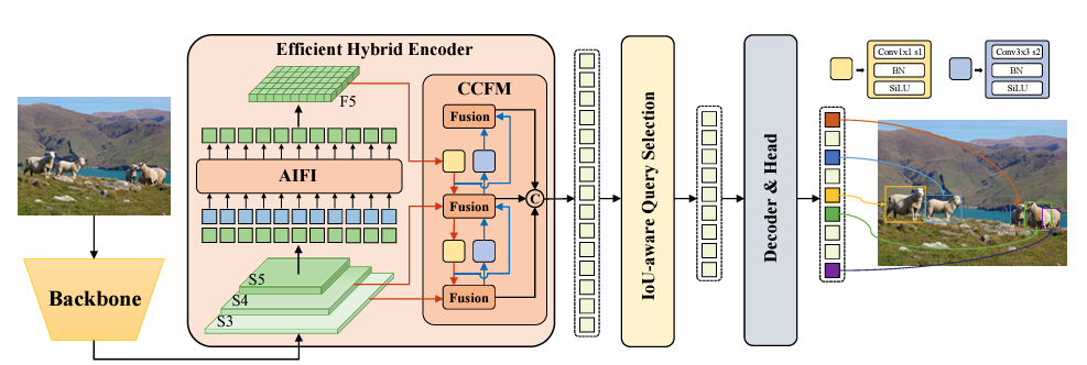
Similar to the YOLO series which provides model versions of different scales through scaling logic, the RT-DETR model also includes two versions: RT-DETR Large (32M parameters) and RT-DETR Extra-Large (67M parameters). The former offers slightly lower performance but has relatively lower requirements for computing resources, making it suitable for deployment on embedded edge devices.

Just like Facebook’s DETR model, the overall architecture of the RT-DETR model also consists of three parts:

A Backbone composed of a convolutional network.
A hybrid encoder.
A decoder and detection head.

The following sections provide a detailed summary and explanation of the structures of the above three parts and the data computation workflow within them.

Backbone

Similar to the DETR architecture, the Backbone in the RT-DETR model serves as the feature extraction engine of the entire model, responsible for extracting multi-scale feature maps (standard DETR models only extract feature maps of the smallest resolution) from the input raw images.

The official implementation of the RT-DETR Backbone supports two network structure options: HGNetv2 and the ResNet series.

The Backbone network of DETR also uses the same ResNet50 and ResNet101. Unlike DETR, which outputs only a single 1/32-scale feature map from its backbone, RT-DETR’s backbone outputs three feature maps of different scales (marked as S3, S4, and S5 in the figure above), corresponding to 1/8, 1/16, and 1/32 of the original image size, respectively. These feature maps contain multi-level information ranging from local textures to global semantics.
HGNetv2 (Higher-order Geometric Network) is a Backbone network structure based on convolutional neural networks developed independently by Baidu. Its core idea is to utilize depthwise separable convolutions and specific structural re-parameterization to enhance accuracy while maintaining low latency.

Regardless of whether ResNet or HGNetv2 is used as the backbone network, once the input image data enters the backbone, it goes through 5 stages (Stage 1-5). With each passing Stage, the height and width of the feature map are halved while the number of channels increases (this is identical to the backbone network of YOLO models). Assuming an input image resolution of 640x640, the outputs of the backbone network are:

Stage 3 (S3): Output feature map size is (C_3, 80, 80) — a scale of 1/8.
Stage 4 (S4): Output feature map size is (C_4, 40, 40) — a scale of 1/16.
Stage 5 (S5): Output feature map size is (C_5, 20, 20) — a scale of 1/32.

Here, C_3, C_4, and C_5 are the number of channels for the three stages, respectively.

Positional Encoding

Regarding positional encoding for feature maps, RT-DETR shares the same calculation formulas and workflows as DETR, with both defaulting to Sine-Cosine Positional Encoding. For a point (x, y) on a feature map, its encoding is generated by sin and cos functions of varying frequencies, generating 128-dimensional vectors for each x and y respectively, which are finally concatenated into a single vector of length 256. For specific calculation formulas and workflows, please refer to the relevant section in Detailed Summary of DETR (DEtection TRansformer) Network Architecture and Computation Workflow.

However, it should be noted that for the feature maps output by the RT-DETR Backbone, only the S5 feature map is flattened into a long sequence. Positional encoding is applied to all pixel points on this lowest-resolution feature map, which is then fed into the Encoder for self-attention computation. This is because RT-DETR considers performing global attention computation solely on the lowest-resolution feature map to be the most cost-effective. The higher-resolution feature maps S3 and S4 directly enter the CCFM module in the hybrid encoder for fusion computation and do not participate in global attention operations, as described below.

Hybrid Encoder: AIFI + CCFM

Next comes the hybrid encoder part of RT-DETR, which is the core component of the model. The design of this part enables the model to balance the global modeling capability of Transformers with real-time performance.

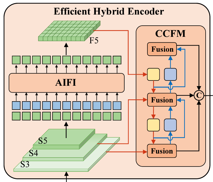
As shown in the figure above, the hybrid encoder mainly consists of two core modules: AIFI and CCFM. The S5 feature map output by the backbone is fed into the AIFI module for processing, outputting the F5 feature map of the same dimensions; meanwhile, the F5 feature map, along with the S4 and S5 feature maps output by the backbone, are sent into the CCFM module for more comprehensive feature fusion.

However, before processing in either AIFI or CCFM, the S3, S4, and S5 feature maps output by the backbone must first undergo dimension alignment.

Dimension Alignment

Why is dimension alignment necessary? This is because the number of channels (C_3, C_4, C_5) output by different stages of the backbone network (such as the aforementioned ResNet or HGNetv2) are inconsistent:

Stage S3 outputs 512 channels
Stage S4 outputs 1024 channels
Stage S5 outputs 2048 channels

In the RT-DETR architecture, to enable feature maps of different scales to be fused via addition in subsequent processing stages and fed into a decoder of uniform dimension, feature maps of all scales must ultimately be unified to the same number of channels (defaulting to 256 in RT-DETR).

Therefore, this step aligns the channel numbers output by different stages to 256. The specific alignment method is straightforward: apply a 1 x 1 convolutional layer to each of the S3, S4, and S5 layers to compress their channel counts from 512/1024/2048 down to 256 channels. After this 1 x 1 convolution, three sets of feature maps with completely identical channel counts (i.e., data dimensions) but different spatial resolutions are obtained.

AIFI

AIFI: Attention-based Intra-scale Feature Interaction. This module is specifically responsible for processing the feature map from the deepest layer and lowest resolution of the backbone (i.e., the minimum-resolution feature map S5 output by the backbone).

The core essence of AIFI is essentially a single-layer Transformer encoder structure, where the input to this encoder is solely the S5 feature map from the Backbone.

Why is self-attention computation unnecessary for S3 and S4? This is because high-resolution feature maps (S3, S4) contain local details, and only the lowest-resolution feature map (S5) contains rich semantic information and global context. Therefore, global interactions only need to be extracted in the low-resolution feature map. Most importantly, the encoder part tends to be the computational bottleneck. If full self-attention computation were performed on feature maps of all scales, the complexity would grow quadratically with the number of pixels. Restricting self-attention computation solely to the lowest-resolution S5 feature map drastically reduces computational cost (FLOPs) while ensuring that the model can extract global relationships among objects in the image.

Following the dimension alignment operation above, the dimension of the S5 feature map input to the AIFI module is (256, 20, 20). The subsequent computation workflow matches that of a standard Vision Transformer Encoder: first, flatten this (256, 20, 20) feature map into a vector sequence of length 400 and dimension 256, and then add positional encoding information to this vector sequence. Regarding positional encoding for feature maps, RT-DETR shares the same calculation formulas and workflows as DETR, with both defaulting to Sine-Cosine Positional Encoding. For specific calculation formulas and workflows, please refer to the relevant section in Detailed Summary of DETR (DEtection TRansformer) Network Architecture and Computation Workflow.

This is followed by standardized multi-head attention computation (defaulting to 8 heads) and feed-forward network (FFN) processing. Finally, the S5 feature sequence processed by AIFI is reshaped back into a tensor shape of (256, 20, 20), which corresponds to F5 in the architecture diagram above.

CCFM

In RT-DETR, CCFM discards the computationally complex self-attention calculations of traditional DETR, turning instead to a CNN-based structure to handle the fusion of feature maps across different resolutions—a concept very similar to PANet used in YOLO. Since it fuses multi-scale features, it naturally includes two fusion pathways:

Top-down: Passing high-level semantic features downward.
Bottom-up: Passing low-level localization features upward.

The core of CCFM performing bidirectional feature fusion lies in its Fusion module, as shown in the figure below.

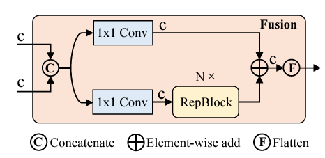
Assume the two feature maps input to the Fusion module are F_high (higher-level features) and F_low (lower-level original features), their channel counts have both been aligned to c, and the resolutions of the high-level and low-level feature maps have been transformed to identical resolutions through previous Upsample or Downsample stages. The workflow of the Fusion module is then as follows:

Feature Concatenate: Concatenate the two input feature maps with channel count c along the channel dimension, outputting a feature tensor with a channel count of 2c.
Feature Splitting: The concatenated feature map with 2c channels enters two parallel branches, each processed by a 1 x 1 convolution to compress the channel count back from 2c to c.
- For the lower branch, an additional sequence of N consecutive RepBlocks is applied. This RepBlock is essentially a 3 x 3 convolution, extracting local spatial features through successive convolutional layers.
Element-wise Add: Element-wise add the base feature map from the upper branch and the enhanced feature map processed by the RepBlock from the lower branch, keeping both the channel count and resolution unchanged.

Therefore, for each Fusion module, the resolution and channel count of its two input feature maps are identical to the resolution and channel count of its output feature map.

For the entire CCFM module, its inputs can be divided into three parts: the output F5 of the S5 feature map processed by the AIFI module, and the dimension-reduced feature maps of the S4 and S3 feature maps from the backbone network. The function to be realized by CCFM is to thoroughly fuse the information from feature maps of three different scales. The fusion method is largely similar to YOLO’s PANet, utilizing UpSample (yellow squares in the diagram below) and DownSample (blue squares in the diagram below) to transform feature maps of different scales to the same resolution, followed by fusion operations within the Fusion Blocks.

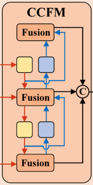
Following bidirectional thorough fusion by the CCFM module, the hybrid encoder finally outputs three fusion-enhanced feature maps from the three Fusion Blocks:

P3 (80 x 80 x 256): Contains rich details, beneficial for detecting small objects.
P4 (40 x 40 x 256): Medium scale.
P5 (20 x 20 x 256): Contains deep semantics, beneficial for detecting large objects.

Finally, these three feature maps undergo flattening operations to obtain three serialized vectors of dimension 256 (6400 x 256, 1600 x 256, and 400 x 256). These three sequences are then concatenated (this is the role of operation C in the CCFM module), ultimately outputting a long sequence of 8400 x 256.

Decoder and Detection Head

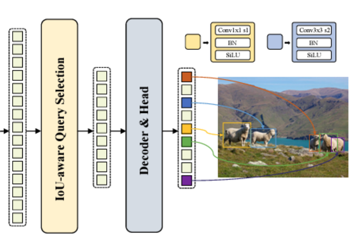
The final part of RT-DETR is responsible for end-to-end object detection based on the 8400 x 256 long sequence (for an image input with 640x640 resolution) output by the previous stage (i.e., the hybrid encoder output). This part is mainly composed of the IoU-aware Query Selection module and the Transformer Decoder. That is, the data output by the hybrid encoder is not directly fed into the decoder; instead, an IoU-aware query selection module first screens it to pick the most promising queries from the encoder’s output as the decoder’s input, thereby reducing the computational load of the decoder.

IoU-Aware Query Selection

The overall working logic of the IoU-aware Query Selection part is: Utilizing the output of the hybrid encoder (8400 x 256), select the Top-K (defaulting to top 300) candidates with the highest predicted IoU quality, which are most likely to be true objects, to serve as the queries for the Decoder.

First, to achieve IoU awareness, RT-DETR designs a lightweight detection head at the output end of the hybrid encoder. This detection head is not a deep network, but an extremely streamlined set of linear prediction layers**.** Taking the 8400x256 long sequence output by the hybrid encoder (which can be considered as three feature maps containing 8400 patches) as input, it uses independent linear prediction layers across 3 separate branches to obtain classification predictions, bounding box predictions, and IoU prediction results corresponding to the 8400 patches.

All three branches map the input 256-dimensional features to their output target dimensions:

Classification branch: Output dimension is 8400 x num_classes, predicting the confidence of each point belonging to each category.
Regression branch: Output dimension is 8400 x 4, predicting the offset (x, y, w, h) of each point relative to its coordinate origin.
IoU branch: Output dimension is 8400 x 1, predicting the IoU quality score between the predicted bounding box corresponding to this point and the potential ground truth box of the detected object.

With the output data from the above three branches, 8400 quality scores can be constructed according to the following formula:

$$ Score = \text{Class_Score} \times \text{Predicted_IoU} $$

The former is the confidence score of the category with the highest confidence value in the classification branch for the current patch, while the latter is the IoU quality score of this patch. Evaluation is performed using this quality score; a point is selected for the subsequent Decoder only when the model is both certain of its category and confident in its ability to box it accurately.

Next, the above 8400 quality scores are sorted in descending order by Top-K, and the 300 with the highest quality scores are selected as the output for this stage. Therefore, through the workflow above, it is equivalent to selecting 300 out of 8400 candidate boxes based on quality scores as the basis for further screening, rather than using all 8400 candidate boxes as alternatives, which drastically reduces the computational workload of the Decoder stage.

Ultimately, the output of the IoU-aware Query Selection module is not a single tensor, but a set of structured information. For each query selected in the Top-K calculation process above, two pieces of information are output at this stage:

Content Query: The 256-dimensional feature corresponding to each feature point. These vectors are used as input to the self-attention module in the next-stage Decoder, with a dimension of 300 x 256.
Reference Points: The coordinate positions (x, y, w, h) output by the aforementioned regression branch, with a dimension of 300 x 4.

Decoder

The structure of the Decoder part remains standard: self-attention module + cross-attention module + feed-forward module. However, to balance computational speed, the cross-attention module here does not adopt the full Cross-Attention of standard Transformers (where every query computes against all 8400 points), but instead adopts Deformable Attention.

Similar to the architecture of a standard Transformer Decoder, the network structure of the RT-DETR model’s Decoder part contains a stacked structure of 6 identical network modules. Each layer contains an independent self-attention computation module + multi-scale sampling cross-attention module + feed-forward network (FFN) module + classification head and regression head composed of linear layers.

Self-Attention Module

The role of this step is to allow sufficient information exchange among the 300 Content Queries.

This self-attention module takes the Content Queries of dimension 300 x 256 as initial input, generates corresponding positional encodings using the Reference Points as references, adds them to the Content Queries, and feeds them into the self-attention computation module. For the computation workflow of the self-attention module, please refer to A Thorough Guide to Understanding the Encoder Structure and Workflow of Transformer Models.

The output of the self-attention module consists of the Content Queries after thorough information exchange, maintaining a dimension of 300 x 256.

Multi-scale Sampling Cross-Attention Module

The input data for the cross-attention module consists of three parts:

The updated Content Queries output by the preceding self-attention module, with a dimension of 300 x 256.
Reference Points representing the position coordinates of 300 prediction boxes, coming from the output of the IoU-aware Query Selection module (for the first decoder layer) or the updated coordinates from the regression head of the previous decoder module (for the subsequent five decoder layers).
Encoder Features, the global feature sequence output by the hybrid encoder part (containing S3, S4, and S5 scales), with a dimension of 8400 x 256.

It should be noted that the cross-attention module in the Decoder part of the RT-DETR model differs from the cross-attention operations in standard Decoders. It does not perform matrix multiplication on all 8400 x 256-dimensional data contained in the Encoder Features; instead, it selectively samples near the centers of the 300 prediction boxes and performs cross-attention computations on the sampled points in the vicinity of each reference point (i.e., Deformable Attention). This significantly reduces the computational complexity of cross-attention, thereby achieving a balance between computational efficiency and accuracy.

The design of this deformable cross-attention module is one of the keys enabling the RT-DETR model to achieve real-time performance.

Regardless, following the computation of this deformable cross-attention module, the output data consists of new Content Query vectors fused with multi-scale local image features, with the dimension remaining 300 x 256.

Feed-Forward Network (FFN) Module

The purpose of this module is to enhance the non-linear expressive capacity of the features, similar to fully connected layers in CNNs.

Just like standard Encoder and Decoder modules, the input data to the FFN module is the Content Queries output by the previous step’s cross-attention computation (with a dimension of [300, 256]).

The computation workflow of the FFN module follows a standard Linear -> ReLU -> Linear structure, where the intermediate dimension is typically expanded (e.g., to 1024 or 2048). The output data consists of deeply mapped Content Queries, maintaining a dimension of [300, 256].

Classification Head / Regression Head

The input data for both is the Content Query output by the previous layer’s feed-forward network module, with a dimension of 300 x 256. They respectively map classification prediction values and coordinate offsets through independent linear layers.

Classification head: Mapped to the target category count num_classes via linear layers. The output data is classification probabilities (Pred Logits), with a dimension of [300, num_classes].
Regression head: Similarly predicts the bounding box coordinate offsets $\Delta(x, y, w, h)$ through linear layers, and then updates these coordinate offsets onto the Reference Points input to the current layer. The Reference Points used by the next module are the values updated by these offsets.

Model Output

The final output of the RT-DETR model comes from the classification head and regression head of the last Decoder block in the Decoder part. These two independent detection heads respectively output the classification judgment values and coordinate values of 300 detection boxes.

Classification head outputs classification prediction scores (Pred Logits): Dimension is [300, num_classes]. Every query gives a score for all categories.
Regression head outputs predicted coordinates (Pred Boxes): Dimension is [300, 4]. These are the final coordinates (x, y, w, h) continuously refined through the 6 Decoder blocks of the Decoder part.

Next, how do we obtain the final detection results presented from these 300 detection boxes?

First, apply Sigmoid processing to the Pred Logits output by the classification head above, converting them into probability values between 0 and 1. Then, use each query’s maximum score across all categories as the confidence score for that box. At this point, we have 300 predicted boxes with category labels and confidence scores.

Next, perform threshold filtering. A confidence threshold (e.g., 0.5) is typically set. The system directly discards all boxes with scores lower than this threshold and outputs detection boxes with confidence scores greater than the threshold.

The key point of this part is that because the Transformer’s self-attention mechanism has already completed deduplication internally (suppressing duplicate queries pointing to the same target), the remaining detection boxes are theoretically high-quality detection results that do not overlap with each other.