Understanding the Working Principles of mmWave Sensing Radar Technology
- 29 Jun, 2026
In essence, radar (originally an acronym for ‘radio detection and ranging’) is a device that detects a target’s distance, velocity, and direction by transmitting electromagnetic waves (radio waves) towards it and then measuring the reflected radio waves.
In the history of radar technology development, the Pulse Method and Frequency Modulated Continuous Wave (FMCW) are two of the most classic and distinct systems. The Pulse Method is the cornerstone of traditional radar (such as large military radar, early weather radar), while FMCW is the absolute mainstream for modern consumer and automotive millimeter-wave radar applications.
This article provides a detailed summary of the working principles of the Pulse Method and the widely applied FMCW mode in the field of millimeter-wave radar.
What is Millimeter Wave?
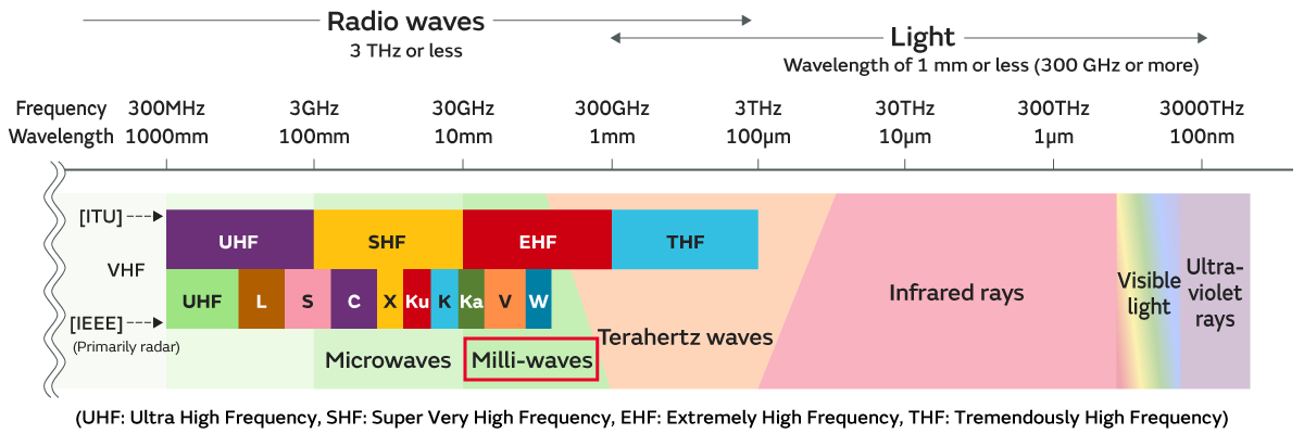
Millimeter wave (mmWave), as the name suggests, refers to electromagnetic waves with wavelengths between 1 mm and 10 mm, corresponding to a frequency range of approximately 30 GHz to 300 GHz. They are called millimeter waves precisely because their wavelengths are measured in millimeters (mm).
In fact, the frequency range of millimeter waves does not have a strict definition. For example, the 26 GHz and 28 GHz bands currently allocated for global 5G communications are also considered millimeter waves.
Currently, in consumer and automotive electronics, the most commonly engineered frequency bands are 24 GHz (gradually being phased out), 60 GHz, 77 GHz, and 79-81 GHz.
The figure below shows the frequency band and wavelength range of millimeter waves in the classification of radio waves. They are called millimeter waves precisely because their wavelengths are measured in millimeters (mm).
Working Principle of the Pulse Method
The working principle and process of the pulse method are quite intuitive. Its core idea is that radar transmits an extremely short, high-power electromagnetic wave pulse, and then passively waits to receive the reflected signal.
It should be noted that in the pulse method operating mode, each extremely short pulse emitted by the radar (e.g., lasting 1 microsecond) contains high-frequency oscillating electromagnetic waves. The frequency of this wave is the carrier frequency, which typically remains constant during the pulse duration. This means that each time the radar transmits, it emits an electromagnetic wave signal with a fixed carrier frequency within this very short period (like the blue pulse in the figure below), and the received echo naturally has the same carrier frequency.
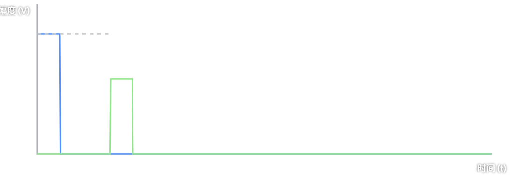
Therefore, the working principle of ranging using the pulse method relies on the time difference (ToF) between the transmitted and received signals. Electromagnetic waves propagate at the speed of light $c$. The radar records the time of transmitting the pulse and the time of receiving the reflected pulse, calculates the time difference $\Delta t$ (i.e., Time of Flight), and then uses the following formula to calculate the distance to the object:
$$ R = \frac{c \cdot \Delta t}{2} $$
For velocity measurement using the pulse method, Doppler Phase Shift is required. The working principle is: if the target is moving, a single pulse can only measure distance, not directly measure velocity. To measure velocity in this scenario, the radar must transmit a pulse train. When the target moves, the round-trip distance for adjacent pulses changes slightly, which causes a change in the phase of the reflected electromagnetic waves. By comparing the received phase difference of consecutive pulses, the radar calculates the target’s radial velocity using the Doppler effect.
How Does Radar Measure the Distance to Multiple Targets Simultaneously?
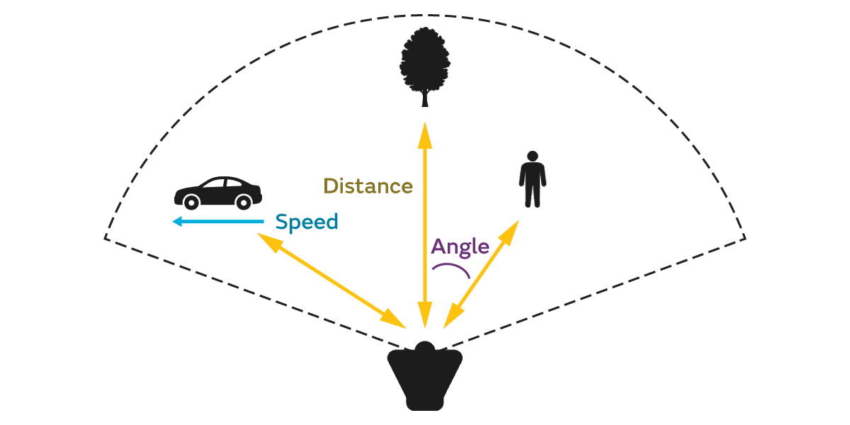
Once the radar pulse is transmitted, the radar receiver remains continuously active, and its corresponding high-speed ADC continuously records the received signal voltage. At this point, all targets within the radar’s coverage area, located at different distances, reflect their respective echoes back to the receiver, causing multiple peaks to appear on the receiver’s voltage curve.
Naturally, there is a concept here called Range Resolution. This concept refers to the radar’s ability to distinguish between two closely spaced objects. For example, in the context of automotive radar detection, if a person is standing very close to a car, will the radar display one large dot or two distinct small dots on the screen? If the distance between them is too close, the echoes received by the radar receiver cannot be distinguished, and they will be perceived as a single target.
As long as the spatial separation between these objects is greater than the radar’s range resolution, the radar receiver will detect distinct, non-overlapping echoes arriving sequentially. The radar’s DSP simply needs to identify the number of peaks on this time axis and their respective timestamps to simultaneously calculate the distances to all targets.
Why Can’t Consumer/Automotive Radars Use the Pulse Method?
This is primarily because: millimeter-wave radar typically requires centimeter-level range resolution.
In pulse radar, to distinguish between two targets, their respective reflected echoes (pulses) must absolutely not overlap on the time axis; that is, the distance between these two targets must be greater than the radar system’s range resolution.
Suppose two objects are separated by a distance $\Delta R$. For the electromagnetic wave to hit the farther object and return, it needs to travel an additional distance of $2 \times \Delta R$. This extra travel time is:
$$ \Delta t = \frac{2 \cdot \Delta R}{c} $$
And for the echo from the first object to completely finish before the echo from the second object begins, the duration of the radar’s transmitted pulse (pulse width $\tau$) must be less than this time difference $\Delta t$.
According to the formula and theory above, if the minimum distance between two targets to be distinguished is 15 cm, then the pulse width emitted by the radar transmitter must satisfy the following condition:
$$ \tau < \frac{2 \times 0.15}{3 \times 10^8} = 1 \times 10^{-9} \text{ 秒} = 1 \text{ 纳秒} $$
However, processing 1 ns signals on low-cost automotive-grade and consumer-grade radar chips presents significant problems:
- The range of radar detection depends on the total transmitted energy (Energy = Power $\times$ Time). If there is only 1 ns to transmit energy, to ensure sufficient echo for electromagnetic waves traveling 100 meters away, the system must unleash instantaneous peak power of hundreds or even thousands of watts within this extremely brief 1 ns. This is not feasible with traditional CMOS-based chips.
- Problems also exist at the receiver end: According to the Nyquist sampling theorem, to reconstruct a 1-nanosecond-wide waveform in the digital domain, the radar receiver ADC’s sampling rate must be at least several GSPS. This is also impractical for low-cost chips used in consumer and automotive electronics, which cost only a few dollars.
- Furthermore, to accurately calculate time differences on the order of tens of picoseconds ($10^{-12}$ seconds) for ranging, the radar system’s internal clock requirements are extremely high. The on-chip clocks (PLL/VCO) must be exceptionally stable with minimal jitter. Such high-precision clock networks are challenging to implement on low-cost SoCs.
This is why, in the fields of consumer and automotive electronics, millimeter-wave radar ultimately abandoned the simpler pulse method and turned to FMCW (Frequency Modulated Continuous Wave).
Working Principle of FMCW Mode
The most prevalent millimeter-wave radar technology in consumer and automotive sectors currently is FMCW (Frequency Modulated Continuous Wave).
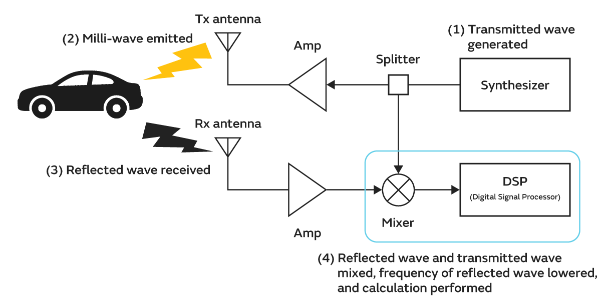
The figure below shows a typical system block diagram of an FMCW millimeter-wave radar:
In FMCW mode, the entire radar system operates as follows:
- Step 1: Transmit Wave Generation. The synthesizer in the system generates a specific frequency millimeter-wave signal. This signal is split into two paths by a splitter: one path goes to the transmit antenna (Tx antenna) for outward transmission. The other path goes to the mixer as a reference signal for subsequent processing.
- Step 2: Millimeter-Wave Transmission. The millimeter-wave signal, amplified by an amplifier (Amp), is transmitted by the transmit antenna towards the target (e.g., a car).
- Step 3: Receive Reflected Wave. The target object reflects a portion of the millimeter-wave signal. The reflected wave is received by the receive antenna (Rx antenna), amplified by an amplifier, and then fed into the mixer.
- Step 4: Mixing and Signal Processing. In the mixer, the received reflected wave is mixed (multiplied) with the reference signal. After filtering out the high-frequency components, a low-frequency Intermediate Frequency (IF) Signal is obtained. This IF signal is then sent to a Digital Signal Processor (DSP), which calculates target information such as distance and velocity.
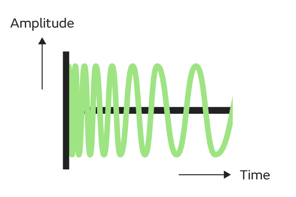
It is important to note that in this mode, millimeter-wave radar does not transmit short electromagnetic pulses like pulse radar. Instead, it continuously and uninterruptedly transmits a continuous wave whose frequency changes linearly with time. This waveform is known as a Chirp (linear frequency modulated pulse).
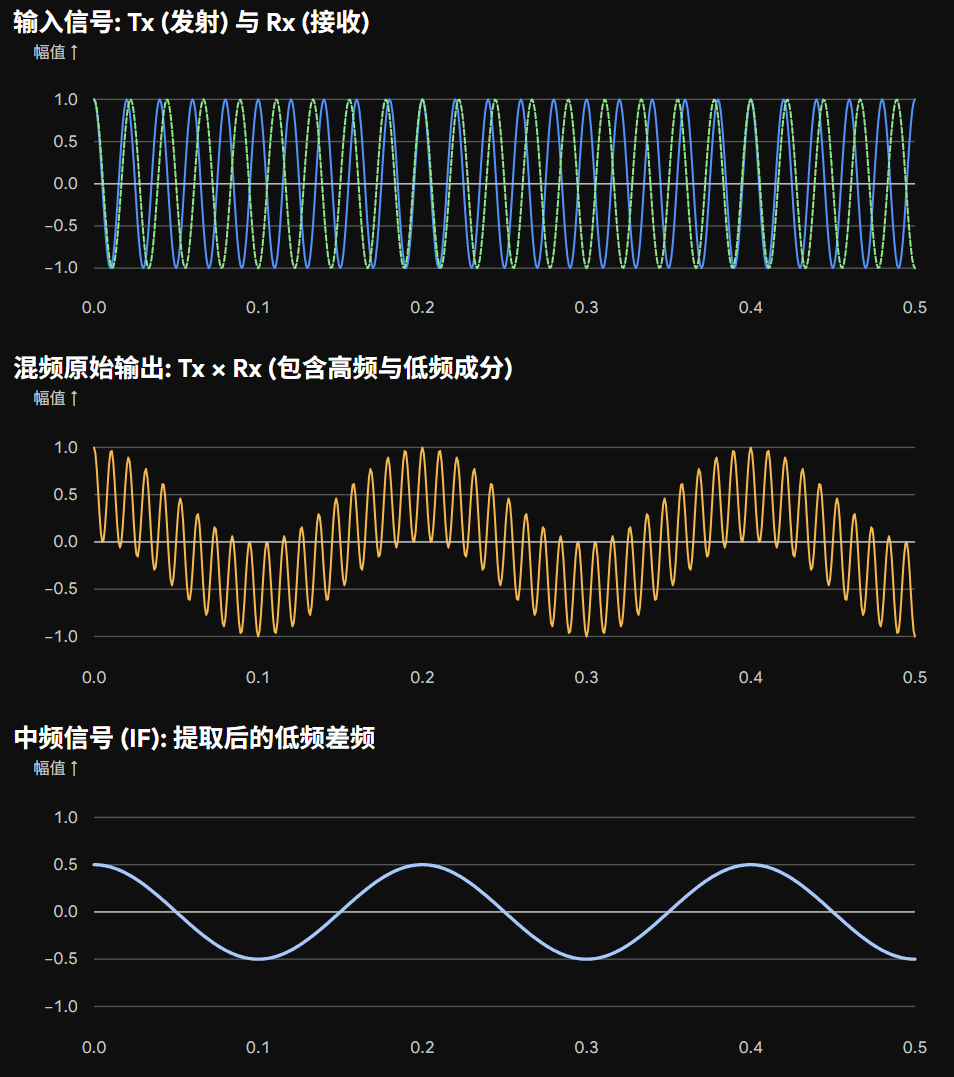
Calculation Process and Working Principle of the IF Signal
For a very brief instant, the transmitted signal (Tx) and received signal (Rx) can be regarded as two high-frequency cosine waves (the same applies to sine waves). Suppose at a certain moment:
• Transmitted Signal (Tx): Frequency is $f_{TX}$ (e.g., 77.005 GHz), expressed as $S_{TX} = \cos(2\pi f_{TX} t)$ • Received Signal (Rx): Frequency is $f_{RX}$ (e.g., 77.000 GHz), expressed as $S_{RX} = \cos(2\pi f_{RX} t)$
For a mixer in radar hardware, its physical function is to perform multiplication on these two voltage signals.
According to the product-to-sum trigonometric identity:
$$ \cos(A) \cdot \cos(B) = \frac{1}{2} [\cos(A+B) + \cos(A-B)] $$
Substituting the expressions for Tx and Rx above, the raw output signal $S_{out}$ of the mixer becomes:
$$ S_{out} = \frac{1}{2} \cos(2\pi (f_{TX} + f_{RX}) t) + \frac{1}{2} \cos(2\pi (f_{TX} - f_{RX}) t) $$
The result of this formula, after multiplying two single high-frequency waves, yields two new waves:
- Sum Frequency Component ($f_{TX} + f_{RX}$): These two frequencies add up to become an ultra-high-frequency signal of approximately 154 GHz.
- Difference Frequency Component ($f_{TX} - f_{RX}$): These two frequencies subtract to become a low-frequency signal of only 5 MHz ($77.005 - 77.000$).
At the output of the mixer, the hardware circuit is always followed by a low-pass filter. The effect of this low-pass filter is to filter out the ultra-high-frequency sum frequency signal, retaining only the difference frequency component. This difference frequency signal is the Intermediate Frequency (IF) signal subsequently used for distance and velocity calculations.
After the above processing, this IF signal is only 5 MHz, which can be easily handled by low-cost processors.
Calculating Distance and Velocity from the IF Signal
The process of calculating distance based on the obtained IF signal is relatively straightforward. Since the IF signal’s frequency is essentially the difference between the transmit and receive signal frequencies, this frequency $f_{IF}$ is perfectly proportional to the target’s distance $R$.
$$ f_{IF} = \frac{2 \cdot S \cdot R}{c} $$
Where $S$ is the Chirp slope ($\text{Hz/s}$), and $c$ is the speed of light.
Thus, after the radar receiver receives the echo signal and samples its generated IF signal, by performing a one-dimensional Fast Fourier Transform (FFT) on the sampled points of each Chirp to convert the time-domain IF signal to the frequency domain and obtain the IF signal’s frequency $f_{IF}$, the distance can be calculated using the formula above. Therefore, a single Chirp signal is sufficient to calculate the target’s distance.
Calculating velocity is slightly more complex, requiring the calculation results from two consecutive Chirp signal sequences.
If the target is moving, due to the very short time interval between two consecutive Chirps, it will generally undergo an extremely small displacement (typically on the micron scale) between successive Chirps. While this minute displacement does not significantly alter the calculated distance, it causes a certain linear shift in the complex phase $\phi$ at the FFT peak for adjacent Chirps.
The phase difference between two adjacent Chirps can be expressed using the following formula:
$$ \Delta \phi = \omega_d \cdot T_c = \frac{4\pi \cdot v \cdot T_c}{\lambda} $$
Where $v$ is the target’s relative velocity, $T_c$ is the Chirp period, and $\lambda$ is the electromagnetic wave’s wavelength.
Therefore, by calculating the phase difference of the FFT peaks from two consecutive Chirp sequences, the target’s relative velocity $v$ can be inversely calculated using the formula above.