Clarifications on Several Issues in the RAG System Workflow
- 16 May, 2026
This article briefly summarizes the overall workflow and module decomposition of Retrieval-Augmented Generation (RAG) systems, and clarifies several issues related to the RAG workflow, vector data storage, and vector retrieval based on this foundation.
Basic Workflow and Core Module Composition of RAG Systems
The following diagram illustrates a typical workflow breakdown of a RAG system:
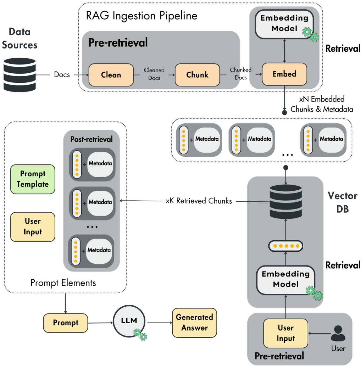
From a module decomposition perspective, a RAG system primarily consists of the following independent modules:
- Indexing: Cleans unstructured documents, splits them into chunks of varying lengths based on semantics, embeds them (i.e., converts them into vectors), and stores them in a Vector Database (Vector DB).
- Retrieval: Calculates the cosine similarity between the user’s query text and the vectors in the database based on the input query message, and recalls the Top-K relevant snippets from the vector database.
- Augmentation: Concatenates the snippets retrieved from the vector database with the original query text to construct an augmented prompt.
- Generation: Feeds the augmented prompt into the LLM, which then generates the final answer based on the augmented context.
The above workflow and module breakdown are simple and straightforward. The rest of this article clarifies several basic concepts regarding the operation of RAG systems to ensure a clearer understanding of all aspects of the system’s operation.
Dimensionality Issues of Stored Vectors in Vector Databases
As shown in the diagram above, documents added to the knowledge base are first split into chunks of varying lengths based on semantics (meaning each chunk contains a varying number of tokens). If the number of tokens in each chunk differs, does it mean that their corresponding embedding vectors will also have different data dimensions?
In reality, regardless of whether the input text (including the user’s query text and the text chunks decomposed from the RAG knowledge base) is long or short (as long as it falls within the model’s maximum context window), the output vector dimension (Dimension) after processing by the same embedding model is always fixed and identical.
Therefore, even if two chunks have different lengths and contain unequal numbers of tokens, the dimensions of the converted vectors remain identical and fixed after passing through the embedding model. This fixed vector dimension matches the token dimension specified by the embedding model.
In the concrete transformation pipeline, whether it is Chunk A of the knowledge base text or the Query, after model dimensionality reduction and feature extraction, the output is always a $1 \times D$ dimensional floating-point array (a 1D vector). For this exact reason, similarity calculations can subsequently be performed between two vectors of completely identical dimensions (i.e., the vector corresponding to the user’s query text and the vector corresponding to a specific chunk in the vector database).
How do texts of different lengths get transformed into vectors of the same length?
This is because the underlying Large Language Model (based on the Transformer architecture) employs a Pooling mechanism in its output layer. The specific implementation consists of the following two steps:
- Token Mapping: Texts of varying lengths are first converted into token sequences, and each token is mapped into a hidden state vector within the model. At this stage, this is an $N \times D$ matrix, where $N$ is the number of tokens and $D$ is the token dimension.
- Pooling (Dimensionality Reduction and Aggregation): The model compresses this $N \times D$ matrix into a $1 \times D$ vector via a specific strategy to represent the global semantics of the entire text segment. Common approaches for this pooling operation include:
- Mean Pooling: Averages the vectors of all tokens across each column.
- CLS Token: Extracts the vector corresponding to the special
[CLS](Classification) token at the beginning of the input sequence, which is trained to represent the semantics of the entire sentence.
Vector Similarity Calculation Logic
As described above, whether it is the user’s query text prompt or the vector corresponding to a knowledge base document segment stored in the vector database, their dimensions are identical at $1 \times D$. When subsequently calculating the similarity between two vectors, the primary logic utilized is Cosine Similarity and Dot Product.
Cosine similarity measures the angle between two vectors in space. Taking vector $A$ (Query) and vector $B$ (Chunk) as examples, both having a dimension of $n$:
$$ \text{Cosine Similarity} = \cos(\theta) = \frac{A \cdot B}{|A| |B|} = \frac{\sum_{i=1}^{n} A_i B_i}{\sqrt{\sum_{i=1}^{n} A_i^2} \sqrt{\sum_{i=1}^{n} B_i^2}} $$
💡 In natural language processing or audio retrieval, the norm (magnitude) of a feature vector often represents the length of the text or the energy level of the audio segment, whereas the direction of the vector represents the true semantics or feature attributes. Therefore, using the cosine similarity formula above decouples the scale from the abstract semantics. The numerator portion ($\mathbf{q} \cdot \mathbf{k}$) is actually the dot product between the two vectors, which measures the absolute overlap between the two tensors across all dimensions. The denominator portion ($|\mathbf{q}| |\mathbf{k}|$) is a scalar acting as a normalization factor to forcibly eliminate scaling errors caused by differences in tensor norms (magnitudes).
For two vectors of the same dimension calculated via the formula above, the result ranges between -1 and 1:
- A result closer to
1indicates that the angle between the two vectors is smaller, meaning the vectors nearly overlap in space, their semantics are very similar, and they represent the perfect target for RAG recall. - A result trending toward
0indicates that the vectors are orthogonal (perpendicular) to each other in space, implying that the two vectors are completely unrelated (i.e., orthogonal), the two text segments discuss entirely different topics, and their feature dimensions do not intersect. - A result close to
-1indicates that the vectors point in opposite directions in space, representing opposite/antonymous semantics. In certain specifically trained embedding spaces, this scenario denotes complete semantic opposition (such as the extremes of good and bad).
The vector database then performs the above calculations between all stored vectors and the user’s query vector based on this formula (or its approximate efficient algorithms, such as HNSW), recalling the Top-K documents with the matching calculation results.
In engineering practice, if all document vectors $\mathbf{k}$ have undergone $L_2$ normalization prior to storage in the vector database (ensuring their magnitudes equal 1), and the query vector $\mathbf{q}$ has also undergone the same normalization operation, the denominator in the formula above becomes 1. At this point, the cosine similarity calculation simplifies into a dot product calculation:
$$ \text{sim}(\mathbf{q}, \mathbf{k}) = \mathbf{q} \cdot \mathbf{k} = \sum_{i=1}^{d} q_i k_i $$
Vector Database Retrieval Workflow
The previous sections outlined the calculation process for finding the vector closest in semantics to the user’s query via the cosine similarity formula between two vectors. However, if the RAG database stores a massive volume of content and a large number of records, performing a cosine similarity calculation against every single record in the database for every retrieval operation would result in an astonishing computational load.
Below is a detailed summary and explanation of the HNSW (Hierarchical Navigable Small World) algorithm, which is the most mainstream algorithm applied in the field of high-speed vector retrieval.
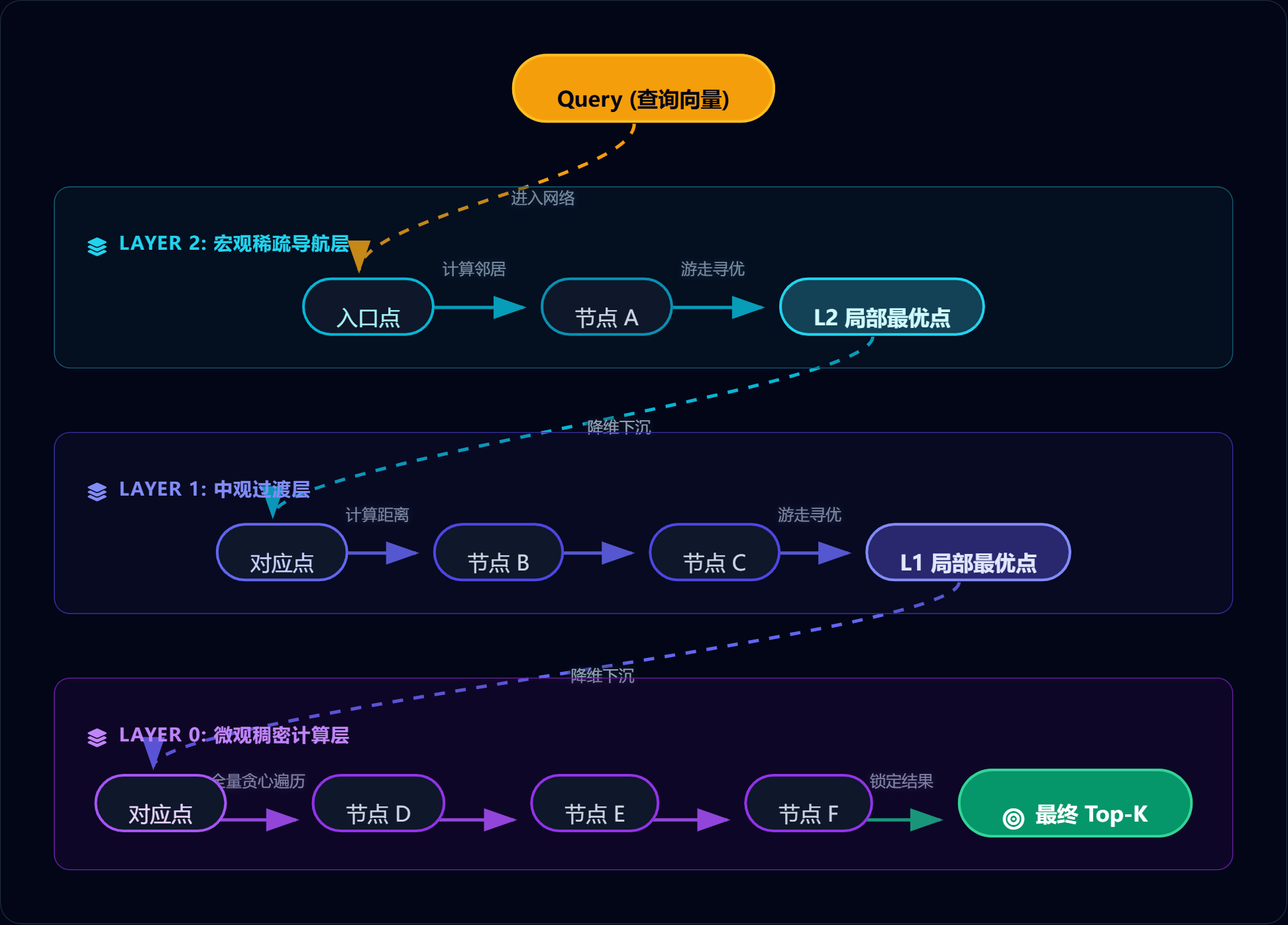
Overall, the HNSW algorithm adopts a multi-layer graph spatial approach to solve the computational and search problems of massive vectors. Under this multi-layer graph structure, nodes in the upper layers are sparse and responsible for quickly locating the general region of the target node, while nodes in the lower layers are dense and responsible for executing fine-grained searches to accurately locate the target node. With this design, the vast majority of nodes are not directly connected, yet any two points can be found in just a few steps.
The multi-layer graph structure essentially places each vector in the vector database into different layers during the indexing stage. Upper-layer nodes contain connection information for the lower layers; thus, during vector retrieval, the system first performs a rough localization via upper-layer nodes, then descends to the bottom layer using the lower-layer connections found within those upper nodes, progressively and precisely locating the nearest neighbor node.
The information contained within each node can be roughly described using the following data structure:
struct HNSWNode {
    int id ;
    float* vector; // Points to the 768-dimensional feature vector
    int max_layer; // The highest layer level this node appears in

    // The three layers are essentially three 1D arrays storing neighbor IDs for each respective layer
    std::vector<int> layer_2_neighbors;
    std::vector<int> layer_1_neighbors;
    std::vector<int> layer_0_neighbors;
};- Layer 2 nodes (i.e., Max Level = 2): Contain connection information for Layer 0 + Layer 1 + Layer 2.
- Layer 1 nodes (Max Level = 1): Contain connection information for Layer 0 + Layer 1.
- Layer 0 nodes (Max Level = 0): Contain connection information for Layer 0 only.
In this scenario, every time a vector search is performed, the system first finds the closest vector Node-Layer-2 in the Layer 2 vector list, retrieves the layer_1_neighbors list saved within Node-Layer-2 to find the closest vector Node-Layer-1 in Layer 1, and subsequently retrieves its corresponding layer_0_neighbors list from Node-Layer-1 to finally identify the Layer 0 vector closest to the target vector from this list.
Therefore, the vector search workflow of the HNSW algorithm roughly mirrors the diagram below. Because practical RAG workflows do not merely return a single record, but rather return Top-K records, a candidate list is often added at each layer during the retrieval process, with the final returned result being the list of the top $K$ vectors closest to the query text vector:
Storage Content of Vector Databases
The next question is: for a RAG vector database, vectors corresponding to all chunks after text splitting are stored within it. In engineering practice, what information does each record in these vector databases typically store?
Generally speaking, a standard vector database record contains at least the following components:
- Primary Key (Primary Key ID): The primary key of the database record, functioning similarly to the primary key in relational databases. The data format is typically
Int64orString (UUID), serving as the unique token for physical storage and in-memory index mapping. - Dense Vector: This is the core content stored in a vector database record. Its data format is a floating-point array (such as
Float32,Float16, orINT8), corresponding to the vector content of each text chunk. Vector retrieval involves calculating the cosine similarity between this dense vector and the vector corresponding to the user’s input prompt text. - Scalar Metadata: Used to store structural attributes accompanying the vector, generally used for attribute filtering (for instance, using this attribute to distinguish which text file a given text chunk originates from). Data types typically include
Int,Varchar,JSON, and others.
As we can see, the records in the vector database mentioned above do not contain the raw text chunk data. In this case, when a vector is found via the cosine similarity algorithm during subsequent vector searches, how does the system locate and retrieve the chunk text corresponding to this vector so that it can be concatenated with the user’s input query prompt?
To address this issue, the most straightforward approach is to store the content of the text chunk directly as a special field (such as a VARCHAR type) within the aforementioned Scalar Metadata portion, keeping it alongside the vector inside the vector database. This way, when the vector is retrieved later, the underlying system can directly return the chunk text string associated with that vector.
However, the problem with this scheme is that the essence of vector retrieval computation is intensive floating-point arithmetic, which requires the feature arrays participating in the calculation to reside in the L3 cache or high-speed RAM. Plain text chunk data is entirely useless for the vector computation process. Loading the entire contents of the vector database (including the aforementioned chunk text content) into memory simultaneously results in severe memory fragmentation and cache misses during computation.
Consequently, mainstream vector databases (such as FAISS and Qdrant) currently store only the [Primary Key, Dense Vector] portion during vector storage, while massive text information such as raw text chunks and metadata (e.g., source document names, page numbers) is stored in a separate, dedicated Key-Value database (such as RocksDB or Redis) or document database (such as MongoDB or Elasticsearch). In this setup, the Primary Key acts as a foreign key connecting the two heterogeneous databases. Once vector retrieval calculations locate the vector, its corresponding chunk text and other metadata can be retrieved from the other database via the Primary Key.