An Analysis of the Network Structure and Output Data of the YOLOv8-Pose Model
- 13 May, 2026
In the article Decoding the Network Architecture of the YOLOv8 Model, I provided a detailed explanation of the network structure of YOLOv8—especially the design and computation process of its detection head—based on the architectural differences between YOLOv8 and YOLOv5. This article focuses on comparing the network structures of YOLOv8 and YOLOv8-Pose, providing a detailed summary and explanation of the detection head, as well as the dimensions and structures of its output data.
Reviewing the Detection Head Structure of the Standard YOLOv8 Model
Let’s state the conclusion first: The Backbone and Neck of YOLOv8-Pose and the standard YOLOv8 model are completely identical. The core architectural differences are 100% concentrated in the Head design, loss function definitions, and corresponding post-processing. Therefore, studying the YOLOv8-Pose model requires a solid understanding of the standard YOLOv8 model, which can be found in Decoding the Network Architecture of the YOLOv8 Model.
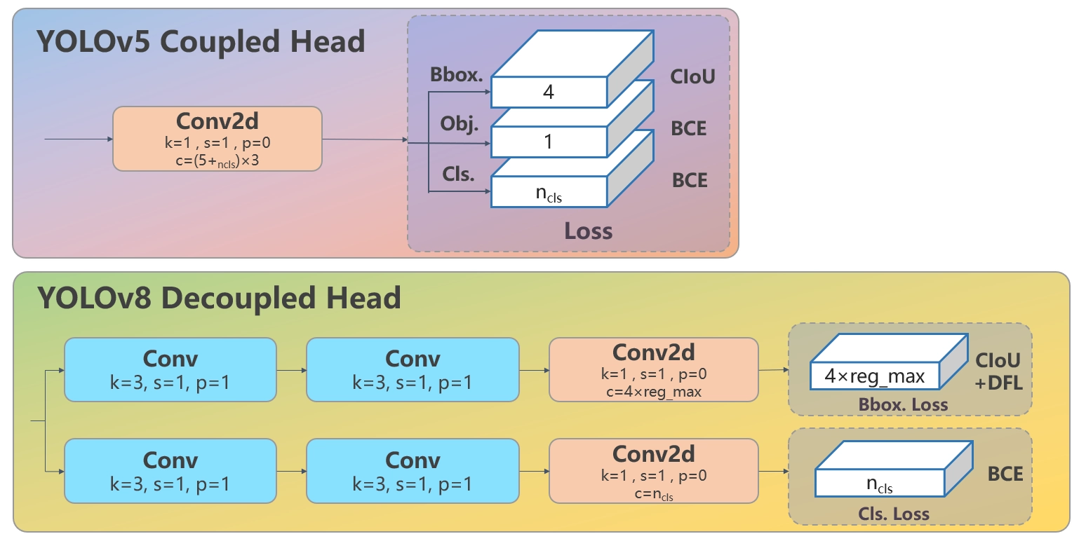
The detection head structure of the standard YOLOv8 model is illustrated in the figure below. Simply put, the Backbone of the network extracts features from the input image, the Neck thoroughly fuses the feature information contained in feature maps of different scales, and the fully fused features are finally fed into the detection head. The detection head of the YOLOv8 model is divided into two independent processing paths: the regression head uses CIoU + DFL (abandoning the Anchor-Based mechanism used in previous generations) to calculate and output bounding box coordinates, while the classification head uses standard BCE to calculate the class probabilities for each bounding box.
Ultimately, the detection head of the YOLOv8 model outputs 8,400 bounding box coordinates and their corresponding class information (with confidence directly taking the maximum value among the class probabilities). During the post-processing stage, valid bounding boxes are filtered out from these 8,400 candidates to form the final detection output.
Detection Head Structure of the YOLOv8-Pose Model
As mentioned above, the difference between the YOLOv8-Pose model and the standard YOLOv8 model lies solely in the Head:
- Standard YOLOv8 Head: The biggest difference from previous generations like YOLOv5 is the adoption of a Decoupled Head, which splits into two parallel branches: the
Box Branch(bounding box regression and DFL) and theCls Branch(classification). - YOLOv8-Pose Head: Evolves into a Tri-Branch structure based on the standard YOLOv8 Head. Building upon the original Box and Cls branches, it adds an independent keypoint branch, the
Keypoint Branch.
The figure below is a schematic diagram of the detection head structure of the YOLOv8-Pose model:
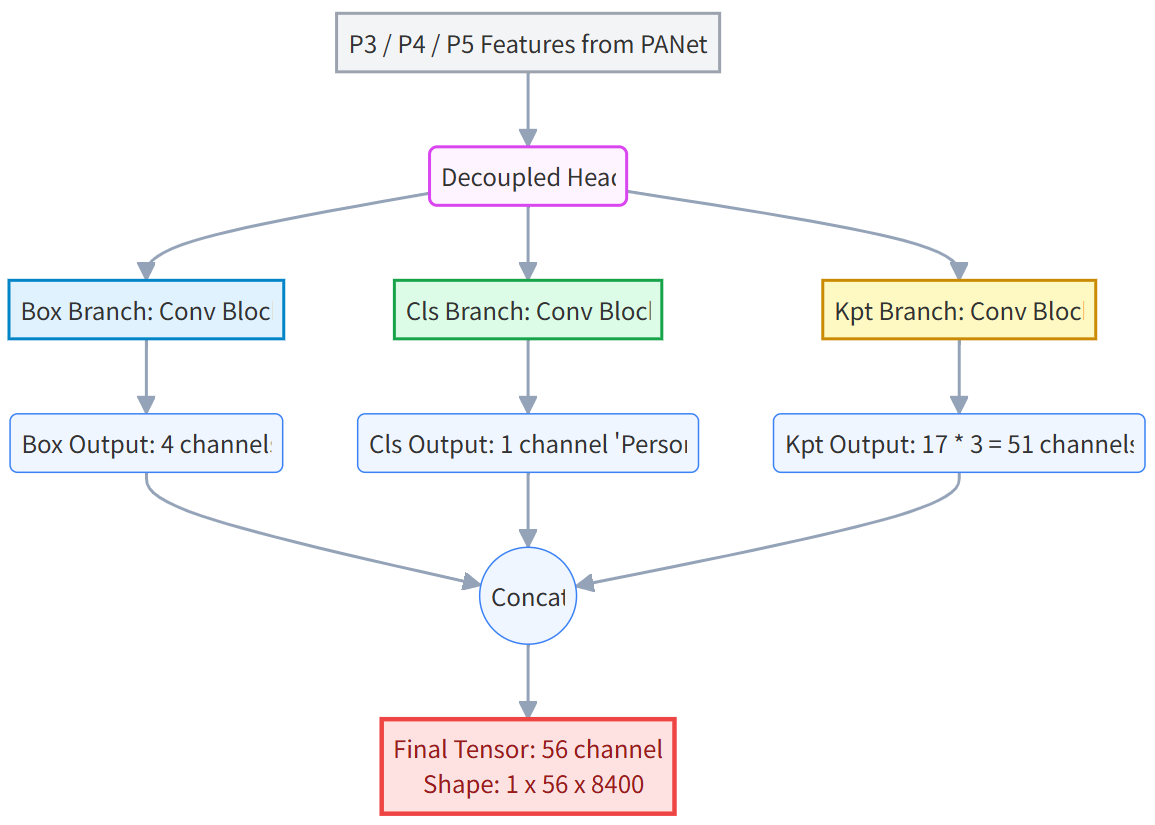
As can be seen, the coordinate regression head (Box Branch) and classification branch (Cls Branch) in the YOLOv8-Pose output head are identical to those of the standard YOLOv8 model. The only difference is that the Pose model introduces an additional, independent, and parallel Keypoint Branch.
YOLOv8 Model Output and Filtering
To understand the filtering logic and post-processing workflow of the YOLOv8-Pose model’s output data, one must first thoroughly understand the post-processing workflow of the standard YOLOv8 model.
The YOLOv8 model is pre-trained on the COCO dataset by default. The COCO dataset contains 80 classes; therefore, for the standard YOLOv8 model, the data dimension of the coordinate regression head for each bounding box is 64 (for details, refer to Decoding the Network Architecture of the YOLOv8 Model), the classification head outputs an 80-dimensional vector for each box (due to the 80 classes), and the feature maps across three scales (P3/P4/P5) jointly output 8,400 bounding boxes. Thus, the total output dimension of the detection head is [8400, 144].
Before entering the NMS post-processing stage, the 64-dimensional data for each bounding box from the regression head is converted into 4-dimensional absolute coordinates (typically $x1, y1, x2, y2$) via DFL integration (Softmax weighted summation). Consequently, the raw output tensor fed into the post-processing stage (including NMS) contains data where each bounding box consists of: 4 dimensions for coordinates + 80 dimensions for class probabilities = 84 dimensions.
At this point, the output dimension of the YOLOv8 model is [8400, 80 + 4]. Next, based on the 80-dimensional class data from the classification branch, a Max operation is applied to retain only the highest class score and its index for each bounding box, using this maximum score as its confidence. The data dimensions then become:
- Coordinates: $8400 \times 4$
- Score: $8400 \times 1$
- Class: $8400 \times 1$
The subsequent post-processing workflow mainly consists of two serial core steps and two thresholds (conf_thres and iou_thres):
- Initial Confidence Filtering: A coarse filter based on the aforementioned confidence score to remove all bounding boxes with a confidence lower than
conf_thres. This eliminates the vast majority of background boxes using minimal computational overhead. - IoU-based Suppression (IoU-based NMS): A refined filtering process that uses the Intersection over Union (IoU) metric (if the IoU between two boxes exceeds
iou_thres, they are considered the same object) to discard redundant boxes for the same object.
The bounding boxes surviving this IoU NMS filtering constitute the final detection output of the model.
YOLOv8-Pose Model Output and Filtering
The YOLOv8-Pose model is pre-trained on the COCO Keypoints (Pose) dataset. In the official annotations of this dataset, only the “person” class has complete annotations for 17 keypoints, while the other 79 classes lack keypoint annotations. Therefore, when Ultralytics officially trains yolov8n-pose.pt, its configuration file (e.g., coco-pose.yaml) hardcodes nc: 1 (Number of Classes = 1, restricting detection to the person class only).
# Train/val/test sets as 1) dir: path/to/imgs, 2) file: path/to/imgs.txt, or 3) list: [path/to/imgs1, path/to/imgs2, ..]
path: coco-pose # dataset root dir
train: train2017.txt # train images (relative to 'path') 56599 images
val: val2017.txt # val images (relative to 'path') 2346 images
test: test-dev2017.txt # 20288 of 40670 images, submit to https://codalab.lisn.upsaclay.fr/competitions/7403

# Keypoints
kpt_shape: [17, 3] # number of keypoints, number of dims (2 for x,y or 3 for x,y,visible)
flip_idx: [0, 2, 1, 4, 3, 6, 5, 8, 7, 10, 9, 12, 11, 14, 13, 16, 15]

# Classes
names:
  0: person
This is why the Cls branch dimension in the official pre-trained YOLOv8-Pose model is 1 instead of 80.
For the keypoint branch output, when using the COCO Keypoints (Pose) dataset, the annotation data includes 17 human keypoints. Each keypoint requires regressing 3 values:
- The coordinate position $x$ on the feature map
- The coordinate position $y$ on the feature map
- The visibility confidence, used to determine whether the point is occluded or outside the image field of view
Consequently, the keypoint branch outputs $17 \times 3 = 51$ dimensions of keypoint data for each bounding box.
So, for the YOLOv8-Pose model, given the addition of a keypoint branch, what is the post-processing logic from model output down to the final NMS-filtered output?
The answer is that during the post-processing logic of the YOLOv8-Pose model, the post-processing workflow pays no attention to what the keypoints look like; keypoints are simply treated as auxiliary data attached to the bounding box. If the box lives, the points live; if the box dies, the points die.
In other words, in the post-processing workflow of the YOLOv8-Pose model, only the outputs of the Box coordinate regression branch and the Cls classification branch participate in the initial confidence filtering and IoU calculation (this part of the workflow is identical to the standard YOLOv8 model). This post-processing procedure ultimately yields the indices of the surviving boxes. When organizing the final output data, these surviving box indices are used to retrieve the coordinates, classes, confidences, and the associated 51-dimensional keypoints of the surviving boxes all at once from the original [8400, 56] tensor.
- After filtering through the post-processing workflow, if 3 person bounding boxes are obtained, the positions of each keypoint for those 3 person boxes will be output simultaneously.
Fundamentally, therefore, the post-processing workflow of the YOLOv8-Pose model is identical to that of the standard YOLOv8 model, with the keypoint branch data simply being “tacked on” during the final output stage.
YOLOv8-Pose Output from a Source Code Perspective
Below is a code snippet for performing inference on image data using the YOLOv8-Pose model:
MODEL_NAME = "yolov8n-pose"  # Options: yolov8n-pose, yolov8s-pose, yolov8m-pose, yolov8l-pose, yolov8x-pose
model = YOLO(MODEL_NAME)
results = model(frame, verbose=False)
annotated_frame = results[0].plot()
The inference result results in the code above is actually a Python list object whose length equals the batch size of the input data. If a single image is fed into the model for inference during each call, the core data of the inference result resides entirely in results[0].
results[0] is an instance of the ultralytics.engine.results.Results class. It acts like a container, packing different sub-objects internally according to the task:
results[0].boxes: Encapsulates all bounding box information filtered by NMS.results[0].keypoints: Encapsulates all keypoint information accompanying the surviving bounding boxes.results[0].orig_img: Stores the raw input Numpy image (primarily used when subsequently callingplotto draw bounding boxes and keypoints on the base image).results[0].names: A mapping dictionary of detection classes (e.g.,{0: 'person'}).
The primary data information and dimensions contained within the bounding boxes (where $N$ is the number of valid detection boxes output by the model) are:
boxes.xyxy: Dimension[N, 4], corresponding to the absolute coordinates of each box: top-leftx1, y1, bottom-rightx2, y2.boxes.xywh: Dimension[N, 4], corresponding to the center coordinates, width, and height of each box (cx, cy, w, h).boxes.conf: Dimension[N], the maximum class confidence score for each of the $N$ boxes.boxes.cls: Dimension[N], the class index corresponding to each of the $N$ boxes.boxes.data: Dimension[N, 6], the raw concatenated tensor arranged sequentially asx1, y1, x2, y2, conf, cls.
The primary data information and dimensions contained within the keypoint data (where $N$ is the number of valid detection boxes output by the model) are:
keypoints.xy: Dimension[N, 17, 2], representing $N$ persons, 17 keypoints per person, with absolute coordinatesx, yfor each point.keypoints.xyn: Dimension[N, 17, 2], normalized coordinates ($x$ divided by image width, $y$ divided by image height), ranging between[0, 1].keypoints.conf: Dimension[N, 17], representing $N$ persons, with visibility/confidence for 17 keypoints per person.keypoints.data: Dimension[N, 17, 3], the concatenated tensor arranged in the orderx, y, conf(i.e., the reorganized form of the aforementioned 51-dimensional data).