Summary of Calculation Workflows for Model FP16 and INT8 Quantization

This article provides a comprehensive summary of the concepts and calculation workflows for half-precision floating-point conversion (FP16) and fixed-point quantization (INT8) applied to models trained in frameworks like PyTorch.

PyTorch Model Training and Storage Format

In mainstream deep learning frameworks such as PyTorch and TensorFlow, the default tensor data type used is FP32 (32-bit floating-point). Therefore, when we define a convolutional layer (nn.Conv2d) or a linear layer (nn.Linear) in PyTorch, the randomly initialized weights, biases, and the activations generated during the forward pass all occupy 32 bits (i.e., 4 bytes, FP32) of memory space by default.

When model training is completed in PyTorch, we use torch.save() to save the model file to the local disk. Because the default tensor dtype during training is FP32, models saved through this standard workflow are also in FP32 format.

However, why are the official YOLO pretrained model files downloaded from Ultralytics FP16 in size and internal parameters rather than FP32?

This is because the official YOLO pretrained model files provided by Ultralytics (such as yolov8n.pt or yolov5s.pt) are forcibly converted to FP16 format before release. The core purpose of this is to significantly save transmission bandwidth and storage space.

Once model training is complete, Ultralytics invokes a classic internal post-processing function: strip_optimizer(). This function calls the model’s .half() method to convert all its weights into 16-bit half-precision floating-point (FP16) format. The general workflow is as follows:

# A typical developer operation to save storage space
model = torch.load('yolo_fp32.pt')
model.half() # Force convert model weights to FP16
torch.save(model.state_dict(), 'yolo_fp16.pt')

Calculation Process of FP16 Half-Precision Conversion

Strictly speaking, converting the storage format of model parameters from FP32 to FP16 is called type casting / downcasting, rather than quantization in the strict sense.

To understand this conversion process, one must first understand the true memory representation of the FP16 and FP32 data types. Both floating-point types conform to the IEEE 754 floating-point binary standard in memory.

The IEEE 754 specification uses scientific notation (e.g., $-12.5$ can be written as $-1.25 \times 10^1$) to represent floating-point data in memory. The specification divides floating-point representation into three regions: Sign, Exponent, and Mantissa/Fraction. The unified mathematical formula for final reconstruction is:

$$ V = (-1)^S \times (1 + M) \times 2^{E } $$

Where:

• Sign bit S: Always the most significant bit (1st bit), where 0 represents a positive number and 1 represents a negative number.
• Exponent E: Immediately follows the sign bit, used to control the magnitude and dynamic range of the number.
• Mantissa M: Used to control the precision of the number and the number of significant digits. In standard binary scientific notation, the digit before the binary point is always 1 (i.e., $1.xxxxx$). Since it is always 1, to squeeze memory to the absolute limit, IEEE 754 mandates that this 1 is not stored in memory. Instead, only the fractional part after the binary point is stored in memory (i.e., $M$ in the formula above), but during computation, the hardware automatically adds that 1 back.

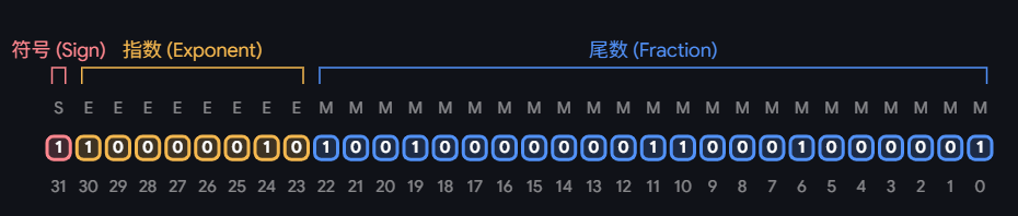
For FP32 and FP16:

• FP32: Single precision, 32 bits, comprising 1 sign bit, 8 exponent bits, and 23 mantissa bits, with a representable data range of $\pm 3.4 \times 10^{38}$.
• FP16: Half precision, 16 bits, comprising 1 sign bit, 5 exponent bits, and 10 mantissa bits, with a representable data range of $\pm 65504$.

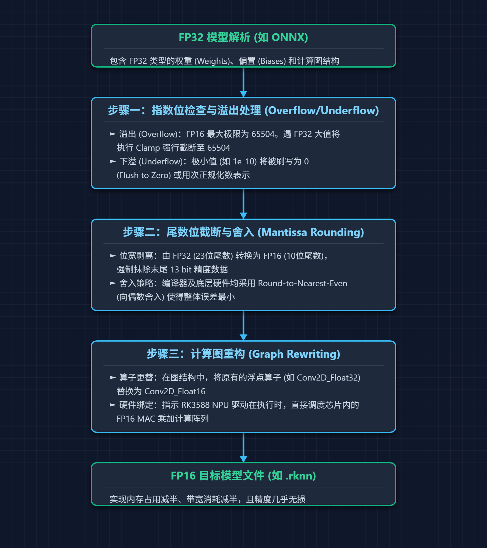
Next, when FP32 parameters saved after model training are converted to FP16 format, what is the specific conversion workflow? It can be mainly divided into the following three steps:

Step 1: Exponent checking and overflow/underflow handling.

• Overflow check: As mentioned above, the maximum absolute value FP16 can represent is 65504. If an FP32 weight value exceeds 65504, the converter typically performs a clamp operation, forcibly truncating the excess value to 65504.
• Underflow check: The minimum normalized positive number FP16 can represent is approximately $6.1 \times 10^{-5}$. If an FP32 parameter value is extremely small, the converter forces it to 0.

Step 2: Forced truncation of the mantissa.

FP32 has a 23-bit mantissa, while FP16 has only 10 bits. During conversion, the converter simply chops off the trailing 13 bits. In binary, this truncation operation is equivalent to erasing tiny significant digits from the 4th to the 7th decimal places. Naturally, this step is the primary source of precision loss in FP32-to-FP16 conversion.

The final step is computation graph reconstruction. This involves replacing the execution logic of operators in the model’s computation graph, swapping out FP32 operators (such as Conv2D_Float32) for FP16 operators (such as Conv2D_Float16).

The complete conversion workflow of the above three steps is illustrated below:

Based on the operations in these three steps, the primary factors that may affect the model’s inference results and precision when converting from FP32 to FP16 stem from two aspects: exponent overflow and forced mantissa truncation. However, in reality, for the vast majority of CV and audio models, the precision loss from FP32 to FP16 is almost negligible. Why is that?

Regarding exponent overflow, whether in CNNs or Transformers, once a model undergoes initial training, the vast majority of its weight parameters $W$ strictly obey a normal distribution with a mean of 0 and an extremely small variance. Furthermore, current CV and audio models are generally equipped with BatchNorm (BN) or LayerNorm (LN) normalization layers. These normalization layers forcibly pull the feature map data distribution back to a standard state with a mean of 0 and a variance of 1 after each convolution or attention mechanism calculation. This means that 99.9% of the weight values in the network fall within the tiny interval $[-2, 2]$. Given FP16’s maximum value of 65504, the probability of exponent overflow on the weight side is practically zero.

The precision loss caused by forced mantissa truncation is mitigated by the rounding strategy adopted during truncation. During the FP32-to-FP16 conversion, a Round-to-Nearest-Even (RNE) truncation strategy is applied to the mantissa bits (this strategy is somewhat similar to round-to-even in decimal systems). If simple direct truncation and discarding were used, the errors would always bias in one direction, causing errors to snowball into a disaster after tens of thousands of accumulations. However, RNE turns truncation error into a symmetrical random noise with a mean of 0. In this case, when the model sums up tens of thousands of product results with zero-mean, independent noise, the positive and negative errors statistically cancel each other out, greatly mitigating the precision loss and error issues caused by forced truncation.

Calculation Process of INT8 Quantization

Unlike FP16, which truncates bit widths based on the IEEE 754 standard, INT8 quantization is a sophisticated mathematical space mapping. It requires cramming the continuous, highly dynamic floating-point space of FP32 into a discrete integer space with only 256 scale levels ($2^8$).

For this mapping, the industry-standard approach is to use linear mapping transformation. This mapping transformation is determined by two key parameters:

• Scaling factor S: An FP32 floating-point value representing the true range in the FP32 space that corresponds to a single scale unit in the INT8 space.
• Zero-point offset Z: An INT8 integer representing which integer scale in the INT8 space corresponds to the absolute zero point in the FP32 space.

Based on these two parameters, assuming the true value in the FP32 space is $R$ and its corresponding quantized value in the INT8 space is $Q$, the fundamental conversion equation between $R$ and $Q$ is:

$$ R \approx S \times (Q - Z) $$

The formula for calculating the quantized value $Q$ from the true value $R$ is:

$$ Q = \text{clamp}\left(\lfloor \frac{R}{S} \rceil + Z, Q_{min}, Q_{max}\right) $$

Where:

• $\lfloor \cdot \rceil$ represents the operation of rounding to the nearest integer.
• $\text{clamp}$ represents the anti-overflow operation, strictly restricting the result within the legal range of INT8 (i.e., between $Q_{min}$ and $Q_{max}$, such as $[-128, 127]$).

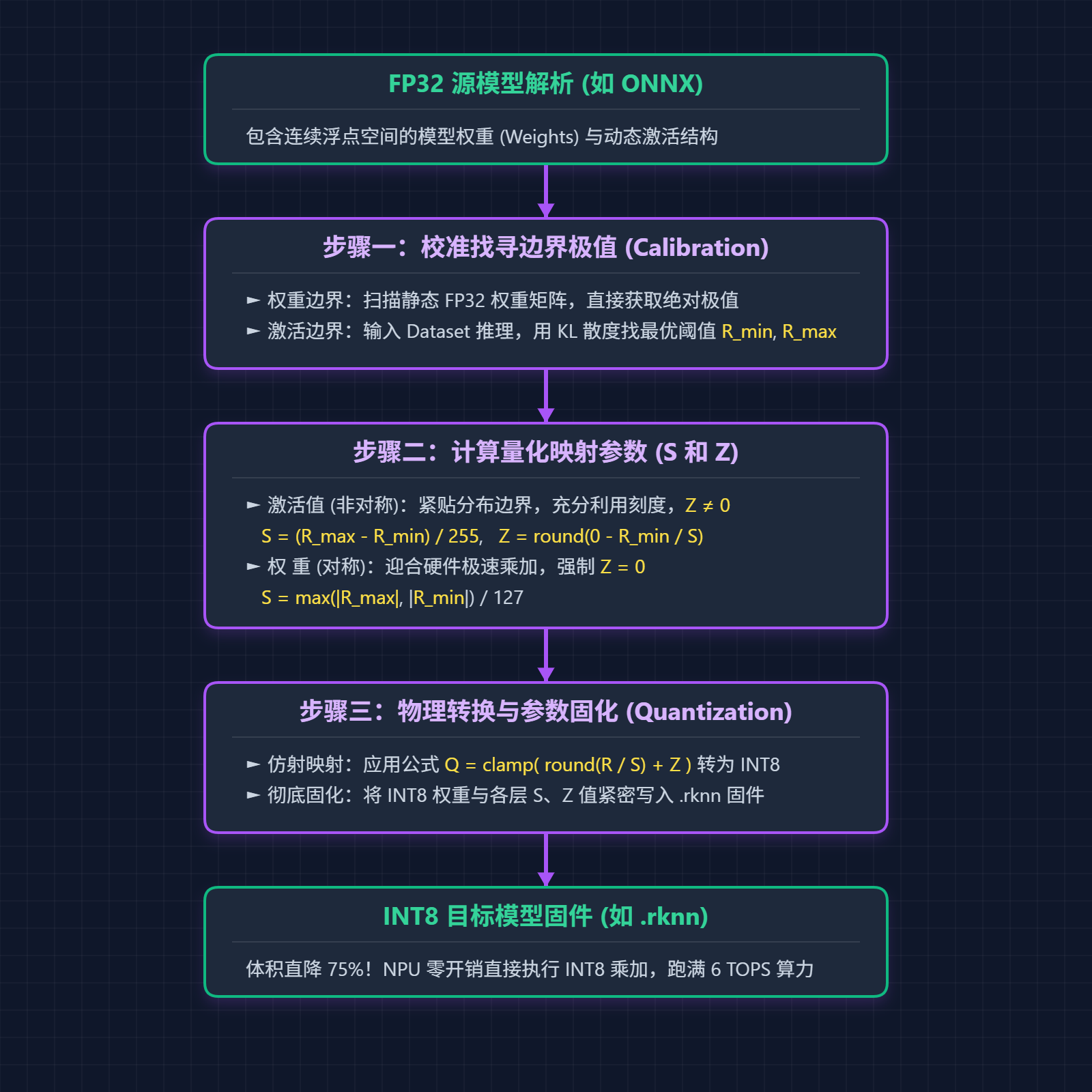
The full workflow for calculating from FP32 to INT8 can also be broken down into the following three steps. In fact, INT8 quantization calculations execute the quantization formula shown above, but before executing this formula, the parameters $S$ and $Z$ must first be calculated.

Step 1: Calculate the scaling factor $S$. Once the range of quantized values $Q$ is determined (a total of 256 scales from -128 to 127 for INT8), the interval range ($R_{max}$ and $R_{min}$) of the true values $R$ in the FP32 space must first be determined. Only then can the range of $R$ be accurately mapped into the range of $Q$.

There are two scenarios here, depending on whether we look at parameter weights/biases or activations:

• For parameter weights and biases: Because these values are constants determined after model training, model converters (such as Rockchip’s RKNN-Toolkit2) can directly scan the convolution kernel matrices in the ONNX file during INT8 quantization to find $R_{max}$ and $R_{min}$.
• For activations: Activations dynamically change with the feature data of input images. This is why performing INT8 quantization requires providing a set of calibration datasets (dataset, typically containing 20-50 representative images) based on the training image set. During INT8 quantization, the model converter uses these images to perform a single forward pass, computes the probability histogram of the output feature maps for each layer, and then uses algorithms like KL-Divergence to find an optimal truncation threshold ($R_{max}$ and $R_{min}$) that best preserves information. Naturally, the $R_{max}$ and $R_{min}$ found this way are derived from the data in our provided calibration dataset, so it is best if the images included in your dataset closely match the actual image formats used post-quantization.

Step 2: With $R_{max}$ and $R_{min}$ calculated in Step 1, parameters $S$ and $Z$ can now be computed. There are two methods for calculating these parameters: asymmetric quantization (for activations) and symmetric quantization (for weights).

Symmetric quantization for weight parameters:

The distribution of weight values produced by model training (i.e., $R_{max}$ and $R_{min}$) is usually centered around 0, being largely symmetrical on both sides. For maximum hardware computation speed, the quantization zero point is strictly required to be $Z = 0$, with the target range of INT8 quantized values set to $[-127, 127]$. For example, if $R_{max}$ and $R_{min}$ are $[-3.5, 3.2]$, the calculated $S$ and $Z$ are:

$$ S = \frac{\max(|R_{max}|, |R_{min}|)}{127} = \frac{3.5}{127} \approx 0.0275 $$

$$ Z = 0 $$

Asymmetric quantization for activations:

Asymmetric quantization can fully utilize all scales of INT8. Assuming $R_{min} = 0$ and $R_{max} = 10.0$, the workflow for calculating $S$ and $Z$ is:

$$ S = \frac{R_{max} - R_{min}}{Q_{max} - Q_{min}} = \frac{10.0 - 0}{255 - 0} \approx 0.0392 $$

$$ Z = \lfloor Q_{min} - \frac{R_{min}}{S} \rceil = \lfloor 0 - 0 \rceil = 0 $$

💡 Why do activations use asymmetric quantization while weights use symmetric quantization? This is because modern CV networks heavily use ReLU family activation functions. After passing through ReLU, all negative numbers in the feature maps are set to 0. If symmetric quantization were forcibly applied to such a single-sided distribution—meaning the center of the mapping range was forced to $0.0$—then in order to represent a number like $15.0$, the quantization scale would have to cover $[-15.0, 15.0]$ and map it to INT8’s $[-127, 127]$. As a result, the 127 states from $[-127, -1]$ in INT8 would never be used (since there are no negative activations), wasting half of the quantization values and effectively turning 8-bit quantization into 7-bit quantization. However, weight distributions are naturally centered around 0 (Gaussian distribution), so using symmetric quantization wastes virtually no space and enables more efficient hardware computation acceleration.

Step 3: Physical conversion and persistence.

Once $S$ and $Z$ are calculated in Step 2, the model converter applies the following formula to convert all FP32 weights into INT8 values, packing them into the quantized model file:

$$ Q = \text{clamp}(\lfloor \frac{R}{S} \rceil + Z) $$

The complete workflow of the INT8 quantization calculation process described above is illustrated in the flowchart below: