A Detailed Explanation of the Concept and Workflow of the BN Layer in Convolutional Networks

This article provides a detailed summary of the theoretical significance of Batch Normalization (BN), which is ubiquitous in various convolutional neural network architectures, and the workflow of BN layer calculations in various computer vision network models.

The Concept and Significance of the BN Layer

Ever since Google proposed Batch Normalization (BN) in 2015, it has become a standard layer in almost all modern CNN architectures (such as ResNet, YOLO, EfficientNet, etc.).

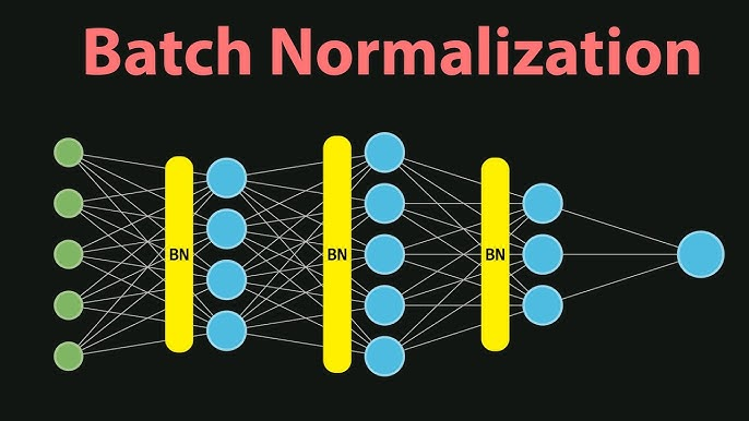
Before the advent of the BN layer, what were the problems associated with training deep neural networks with dozens of layers?

• Extreme sensitivity to weight initialization: If the initial weights were set slightly too large or too small, the output values would either explode or vanish after propagating through multiple layers. Consequently, researchers back then had to spend immense effort studying complex parameter initialization methods.
• Unusably small learning rates: To prevent network parameters from collapsing during training, learning rates had to be set conservatively (e.g., 0.0001), resulting in extremely long training times and low efficiency.
• The vanishing gradient problem: Network designs around 2015 commonly used Sigmoid or Tanh as activation functions. If the input data was too large or too small, it easily fell into the saturation zones of these activation functions (where the curve becomes extremely flat), causing gradients to drop to nearly zero (vanishing gradients), which completely halted network learning.

The root cause of these problems is a phenomenon known as Internal Covariate Shift (ICS). While ICS sounds complicated, it describes a simple issue: during training, when parameters in the first layer are updated slightly, this minor change is exponentially amplified as it propagates through the second, third, and all the way to the one-hundredth layer. As a result, for deep networks, the statistical distribution of input data received at each layer varies drastically and irregularly, making it impossible to learn any consistent patterns from these wildly fluctuating values.

To address these issues, the BN layer introduced a direct solution: Since the data distribution coming from upstream is always unstable, we insert an extra processing step before each layer to forcefully shuffle and normalize the upstream data into a standard format.

Specifically, regardless of the statistical shape of the data passed from the previous layer, the BN layer computes the mean and variance of the current complete training batch (the so-called Mini-batch) and forcibly pulls the input data into a standard normal distribution with a mean of 0 and a variance of 1. Under this mechanism, no matter how deep the network is, every layer can be certain that the data received from the preceding layer conforms to a standard normal distribution.

The question is: If we forcefully transform the input data from the previous layer into a normal distribution with a mean of 0 and a variance of 1, wouldn’t that destroy the feature discriminability that the preceding network layers worked so hard to learn?

To solve this problem, after the normalization calculation, an additional linear transformation step and two learnable parameters, $\gamma$ (Scale) and $\beta$ (Shift), are introduced to restore the network’s expressive power. This hands the choice of “whether input data needs to be normalized” and “the degree of normalization” back to the network for it to learn and decide on its own. The specific calculation workflow is described below.

Another question is: Where is the BN layer typically placed within a CNN network?

The answer is that the BN layer is generally sandwiched between linear operations (such as convolutional layers) and non-linear activation functions (such as ReLU), as shown in the diagram below:

This is because the data produced after a convolution operation is often very scattered in its statistical distribution. By using a BN layer to cluster the data around 0 before passing it into the activation function, the data is perfectly positioned in the most sensitive and effective region of the activation function, thereby obtaining maximized and healthy gradient feedback.

Calculation Workflow of the BN Layer

Generally speaking, the core operations of a BN layer comprise two phases: the Normalization calculation phase and the Affine Transformation phase.

In terms of the workflow, for a given feature $x_i$ within a Mini-batch, the BN layer first computes its mean $\mu_{\mathcal{B}}$ and variance $\sigma_{\mathcal{B}}^2$, and then performs normalization. The normalization maps the input data to a zero-centered, unit-variance linear space. Finally, two learnable parameters, $\gamma$ (Scale) and $\beta$ (Shift), define a new linear mapping to restore the network’s expressive power.

💡 Therefore, no matter how fancy the BN layer might look during training, both phases of its calculation are ultimately linear transformations. Mathematically, the entire processing of input data by the BN layer remains a simple linear transformation: $y = W_{new} x + B_{new}$.

The complete formulas and calculation workflow of the BN layer are as follows: the first three formulas represent the normalization process, and the final formula represents the affine mapping.

$$ \mu_{\mathcal{B}} = \frac{1}{m} \sum_{i=1}^{m} x_i $$

$$ \sigma_{\mathcal{B}}^2 = \frac{1}{m} \sum_{i=1}^{m} (x_i - \mu_{\mathcal{B}})^2 $$

$$ \hat{x}i = \frac{x_i - \mu{\mathcal{B}}}{\sqrt{\sigma_{\mathcal{B}}^2 + \epsilon}} $$

$$ y_i = \gamma \hat{x}_i + \beta $$

From a data dimensionality perspective, the dimensions of the input and output data remain completely unchanged, and the structural semantics are fully preserved. During normalization, the computation is always performed per channel of the input feature map. In other words, when calculating the mean and standard deviation for a single channel, it aggregates all pixel points across all $N$ images in that specific channel.

💡 Why normalize per channel? Because in a CNN, each channel represents an independent and specific semantic feature. Normalizing each channel independently preserves the physical independence between different features, preventing two distinct semantic features from being forcefully averaged together.

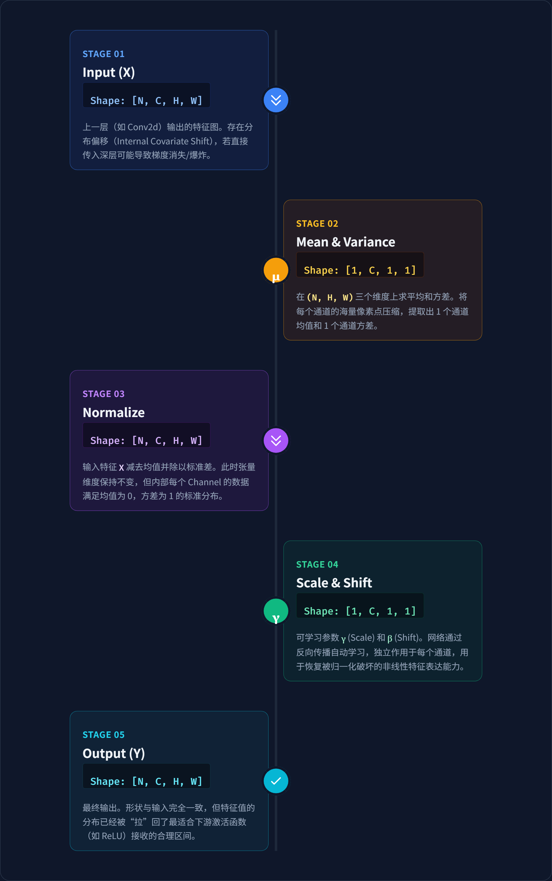
The diagram below illustrates the data dimensions at each stage of the BN layer calculation in a standard CNN network:

• Stage 1: The input data is the feature map output by the previous convolutional layer, with dimensions $[N,C,H,W]$.
• Stage 2: Taking the channel as the unit, extract the feature maps of a specific channel across $N$ images, and compute the mean and variance for all data in these $N$ feature maps, resulting in $C$ means and variances.
• Stage 3: Still operating per channel, normalize the pixels of each feature map in that channel based on its corresponding mean and variance, converting the feature map data of each channel into a standard distribution with a mean of 0 and a variance of 1.
• Stage 4: In the affine mapping stage, each channel has a set of learnable parameters $\gamma$ and $\beta$ learned during training, which are used to linearly map the feature map of that channel.
• Stage 5: The final output data shape remains consistent with the input.

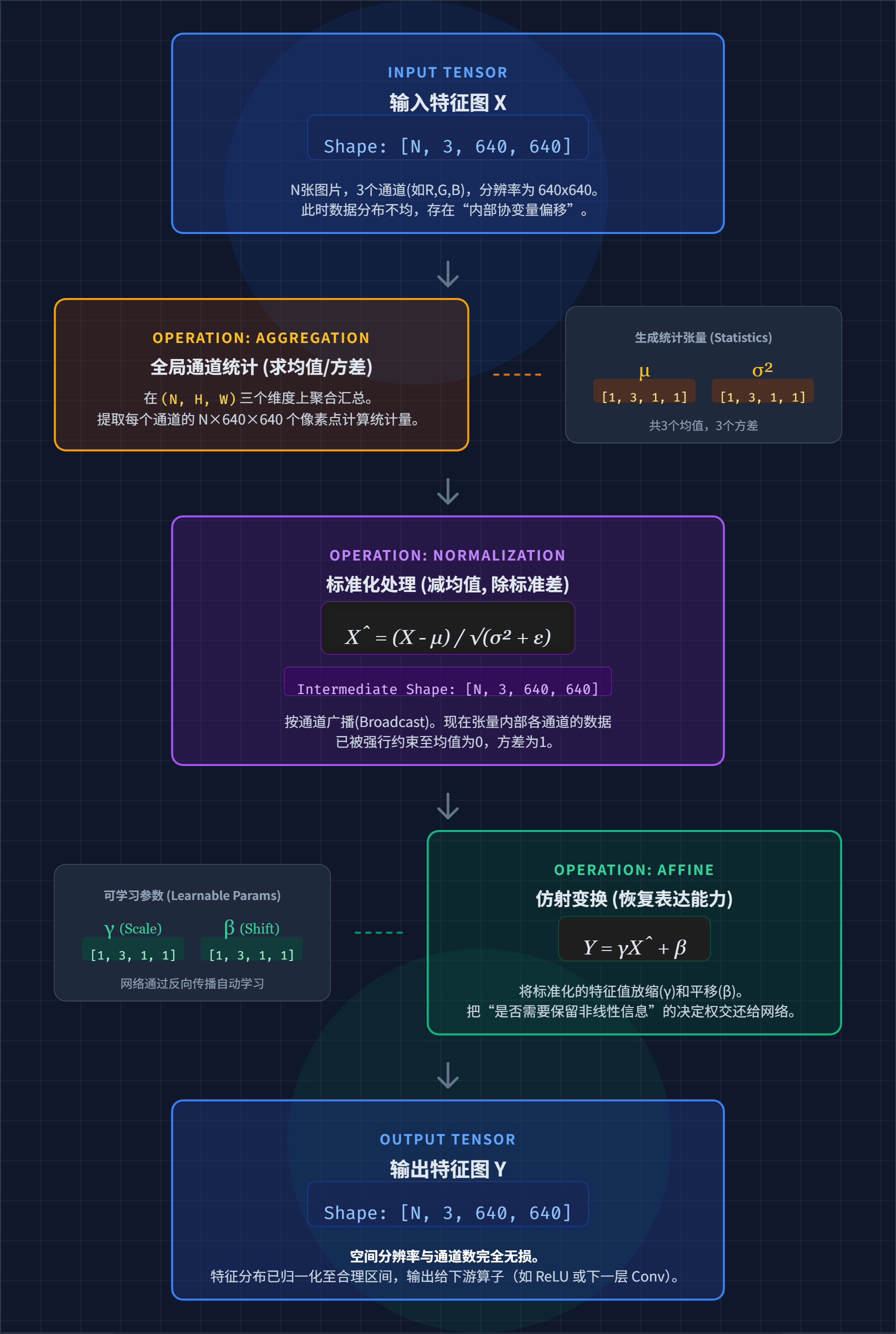
To further clarify the calculation workflow, the diagram below illustrates a complete BN layer operation taking a batch of $N$ images with 3 channels and a $640 \times 640$ resolution as input:

• Throughout the computation, because the input data has 3 channels, the input batch has 3 sets of means and variances, as well as 3 sets of learnable parameters $\gamma$ and $\beta$ corresponding to the three channels.
• Note that this diagram is for illustrative purposes only. The BN layer in CNNs rarely acts directly on the raw input images. For raw images ($[N, 3, 640, 640]$), constant values (such as ImageNet’s global mean and standard deviation) are typically used directly during the preprocessing stage for mean subtraction and division by standard deviation. The true domain of the BN layer is on deep feature maps within the network, processing the outputs of convolutional layers.

Behavior of the BN Layer During Inference

It is important to note that the behavior of the BN layer differs completely between training and inference.

During the forward pass of training, the code calculates the true statistics $\mu_{\mathcal{B}}$ and $\sigma_{\mathcal{B}}^2$ based on the current Mini-batch. Meanwhile, to prepare for inference, the BN layer quietly maintains running averages of the mean (running_mean) and variance (running_var) in the background.

During inference (i.e., model.eval() mode), the BN layer no longer computes batch-specific statistics (since inference inputs might consist of just a single image, causing unstable results if batch size varied). Instead, it directly uses the accumulated running_mean and running_var from training for normalization.

Similarly, the learnable parameters $\gamma$ (Scale) and $\beta$ (Shift) in the affine transformation phase are fixed during inference. Therefore, the linear operations of the BN layer can be mathematically and equivalently fused into the weights ($W_{conv}$) and bias ($Bias_{conv}$) of the preceding convolutional layer.

$$ W_{fused} = W_{conv} \times \frac{\gamma}{\sqrt{\text{running_var} + \epsilon}} $$

$$ Bias_{fused} = (Bias_{conv} - \text{running_mean}) \times \frac{\gamma}{\sqrt{\text{running_var} + \epsilon}} + \beta $$

Consequently, when exporting to ONNX, tools like ONNX-Simplifier are typically used in combination. This process automatically fuses Conv and BN layers, meaning independent BatchNorm nodes will generally no longer appear in the exported *.onnx model graph.