Summary of Audio FFT Calculation Workflow and Spectrum Interpretation
- 28 Mar, 2026
This article summarizes the principles, parameters, and calculation workflows for performing FFT on speech signal sequences to obtain their corresponding spectra. It also provides a Python example to compute and interpret the spectrogram of a WAV file.
Introduction to Speech Signal FFT Calculation and Parameter Summary
As is well known, in the time domain, an audio signal is a pressure value that fluctuates over time (i.e., sound pressure, manifested as amplitude). The principle of Fourier transform proves that any periodic signal can be decomposed into the sum of a series of sine/cosine waves with different amplitudes, frequencies, and phases. Therefore, the fluctuations exhibited by an audio signal in the time domain can also be viewed as being superimposed by countless sine waves with different frequencies, amplitudes, and phases. The FFT (Fast Fourier Transform) calculation performed on a digital audio signal sequence is essentially the extraction of the corresponding combination of various sine waves from this digital audio signal sequence, which is the so-called spectrum.
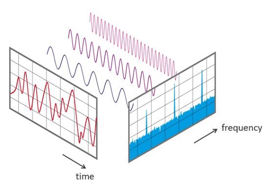
The FFT calculation performed on the discrete-time sequence of an audio signal in the digital domain has the following characteristics:
- The result of performing an FFT calculation on an audio signal sequence is not a continuous frequency analysis. Instead, the total frequency range (from $0\text{Hz}$ to the audio sampling rate $f_s$) is evenly divided into $N$ small blocks, with each block called a Bin. The width of each Bin is $\Delta f = \frac{f_s}{N}$.
- The output result of the FFT calculation is a complex number $(a + bi)$. To obtain the final spectrogram, it is also necessary to calculate the magnitude of the complex number: $\sqrt{a^2 + b^2}$. This magnitude represents the energy level of the frequency component in the signal.
- For real-valued audio signal sequences, the FFT calculation result is symmetric. That is to say, if 1024 audio sampling points are input for FFT calculation, among the 1024 output complex numbers, the first 512 cover information from 0 to $f_s/2$ (the Nyquist frequency), and the last 512 points are merely a mirror image of the first half. Therefore, when plotting the spectrogram, usually only the first $N/2$ data points are taken.
Correspondence Between FFT Calculation Results and Frequency Domain Bins
As mentioned above, for an FFT calculation performed on an audio sequence of length $N$, the calculation result is a complex number sequence of length $N$, where the first half and the second half exhibit mirror symmetry. The entire frequency band corresponding to the FFT calculation result is $[0, f_s/2]$. Because the entire calculation result sequence is mirror-symmetric from front to back, this frequency range is evenly divided into $N/2$ parts.
For each output point of the FFT calculation (called a Bin), the formula for calculating its corresponding frequency point is:
$$ f(k) = \frac{k \cdot f_s}{N} $$
where $k$ is the index of the complex number in the array (starting from 0). If the sampling rate $f_s = 44100\text{Hz}$ and the FFT length $N = 1024$:
- Index 0: $0\text{Hz}$ (DC component)
- Index 1: $1 \cdot 44100 / 1024 \approx 43.07\text{Hz}$
- Index 2: $2 \cdot 44100 / 1024 \approx 86.13\text{Hz}$
- …
- Index 512: $512 \cdot 44100 / 1024 = 22050\text{Hz}$ (Nyquist frequency, i.e., the maximum analysis frequency)
The amplitude of each frequency point is obtained by calculating the magnitude of the complex number corresponding to that frequency point: $\sqrt{a^2 + b^2}$. This magnitude represents the energy size of the frequency component in the signal.
Key Parameters of FFT Operation
The key parameters for performing FFT operations on audio sequences are as follows: (You can understand these parameters in conjunction with the FFT spectrum calculation workflow described below)
- FFT Size / Window Length ($N$): The number of sampling points in each audio sampling frame participating in the calculation, usually a power of 2 (e.g., 512, 1024, 2048, 4096).
- Sampling Rate ($f_s$): The number of samples collected from the analog signal per second. This collection frequency directly determines the bandwidth of the spectrum. According to the Nyquist sampling theorem, the relationship between the maximum frequency that the sampled sample sequence can analyze and the sampling frequency is $f_{max} = f_s / 2$. Therefore, if you want to analyze high frequencies of $20\text{kHz}$, the sampling rate must be greater than $40\text{kHz}$.
- Window: To reduce spectral leakage, it is necessary to window the signal before performing the FFT calculation. The main types of windows include: Hann, Hamming, and Blackman.
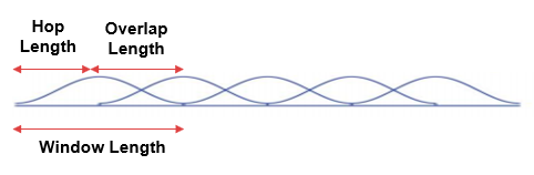
- Hop Size: The sliding distance between two adjacent FFT windows. The more consecutive audio frames overlap (the smaller the Hop Size), the smoother the generated spectrogram will be on the time axis, and the less information will be lost (because window functions attenuate edge energy, which can be compensated through overlapping). However, the smaller the Hop Size, the more frames need to be calculated for the same audio sequence, and the computational cost increases linearly.
A schematic diagram of the audio sampling frame Window Size, sliding window Hop Size, and Overlap Size between two consecutive frames is shown below:
Speech Signal Spectrum Calculation Workflow
To generate a corresponding spectrogram for a speech file, the following steps and workflow are generally required.
Speech Signal Acquisition and Framing
Audio sampling equipment (MIC) acquires analog speech signals at a fixed sampling rate $f_s$ (e.g., 16K, 32K, 44.1K). According to the Nyquist sampling theorem, the maximum frequency that can be calculated and analyzed via subsequent FFT corresponds to $f_s / 2$.
In addition, a speech signal may be several minutes long, and directly performing an FFT on the entire file is meaningless because the frequency of a speech signal constantly changes over time. Therefore, before performing the FFT calculation, the complete speech signal sequence must first be cut into many small segments, each of which is called an audio frame. Typically, the length of an audio frame is $N$ (which is actually the number of points for a single FFT calculation, i.e., the FFT Size), chosen as a power of 2, such as 512, 1024, or 2048.
Of course, in terms of framing, two consecutive audio frames will partially overlap. For example, the first audio frame corresponds to audio samples in the 0-1023 range, the second audio frame corresponds to samples in the 320-1352 range, and so on, until the end of the entire audio file.
Windowing
Every framed audio frame needs to be windowed before performing the FFT calculation. When performing an FFT calculation on an audio sequence without windowing, it defaults to a rectangular window, which leads to spectral leakage and aliasing. The purpose of windowing is to make the amplitude of a signal frame taper off to 0 at both ends, which makes the peaks on the spectrum thinner and less likely to blur together, thereby mitigating the effects of spectral leakage and aliasing. Of course, in this case, the parts at both ends of a signal frame are attenuated and do not receive as much emphasis as the central part. The remedy for this is to have two consecutive audio frames overlap with each other. The time difference between the starting positions of adjacent frames is called the hop size (i.e., Hop Size).
The following figure shows the window functions commonly used in speech signal processing:
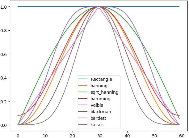
Windowing refers to pointwise multiplication of the audio frame $x[n]$ with a window function frame $w[n]$ of the same length:
$$ x_{windowed}[n] = x[n] \cdot w[n] $$
As a result, the beginning and end of this signal frame are smoothly attenuated to 0, which forcibly achieves continuity at the ends, eliminates discontinuities, and avoids jumps caused by inconsistent amplitudes at the start and end points of the signal sequence.
FFT Calculation and Spectrogram
Next, the windowed digital signal sequence is subjected to FFT calculation. During the calculation, the computational complexity of $O(N^2)$ is reduced to $O(N \log N)$ through efficient butterfly computation methods using odd-even decomposition.
For an audio digital sequence of length $N$, the result of the FFT calculation is a complex number sequence of the same length $N$. As mentioned earlier, because the audio digital sequence consists entirely of real numbers, this complex number sequence of length $N$ exhibits mirror symmetry.
$$ X[k] = \text{Real} + j \cdot \text{Imag} $$
Then, calculate the magnitude of each frequency point: $|X[k]| = \sqrt{\text{Real}^2 + \text{Imag}^2}$, which represents the intensity of that frequency component. Because the energy distributed across various frequency bands of audio spans an extremely large range, it must be converted into decibel values using logarithmic mapping (dB) for representation: $20 \cdot \log_{10}(\text{Magnitude})$.
Finally, by arranging the frequency decibel energy distribution calculated for each frame (vertical axis, using color to represent energy magnitude) in chronological order (horizontal axis), a linear spectrogram is obtained.
Mel-Scale Spectrogram
In the field of digital audio, for tasks like speech recognition or music analysis, ordinary linear frequencies are typically converted into the Mel Scale. This is because the human ear is more sensitive to changes in low frequencies than high frequencies, and the Mel scale better simulates human auditory perception.
The frequency distribution on the frequency axis of a linear spectrogram is uniform, whereas the frequency axis of a Mel-scale spectrogram is sparse at the front and dense at the back—its low-frequency portion is very sensitive, while its high-frequency portion is heavily compressed. Human hearing is non-linear and more sensitive to low-frequency signals; we can easily distinguish the pitch difference between $100\text{Hz}$ and $200\text{Hz}$, but if two frequencies are $10000\text{Hz}$ and $10100\text{Hz}$ respectively, although they also differ by $100\text{Hz}$, the human ear can hardly tell any difference.
The definition of the Mel scale is precisely designed to make equidistant Mel frequency changes feel equidistant in human auditory perception.
The conversion from a linear spectrogram to a Mel spectrogram is not a simple coordinate axis stretching, but rather a re-weighted aggregation of linear frequency energy through a set of Mel Filter Banks. Its general workflow is as follows:
- First, a series of triangular filters are placed on the spectrum: in the low-frequency region, these triangles are narrow and densely arranged; in the high-frequency region, these triangles become wide and sparsely arranged.
- Multiply the amplitude data of the entire frequency band of an audio frame with each triangular filter and sum them up: the first filter will collect the energy of the low-frequency region and output a single value; the last wide filter will collect the energy of a large range in the high-frequency region and output a single value after summation. This yields the Mel-scaled energy distribution for this audio frame.
- Perform the second step processing for all audio frames to obtain the Mel-scaled energy distribution across different frequency bands for all audio frames.
Ultimately, the number of frequency points on the Mel spectrogram depends on the number of Mel filter banks. If there are 1024 linear frequency points in the previous linear spectrogram, passing through 40 Mel filters leaves only 40 Mel frequency points. In this way, the horizontal coordinate of the Mel spectrogram remains the same as that of the linear spectrogram, both corresponding to the number of audio frames; its vertical coordinate becomes the number of Mel filter banks, which is 40, ranging from low to high frequencies.
Example of Speech Signal Spectrum Calculation
Below, taking a phone call speech file R9_ZSCveAHg_7s.wav that comes with the speech classification model (PANNs) code as an example, the Spectrogram and LogmelFilterBank classes from the torchlibrosa library are used respectively to generate the linear spectrogram and Mel-scale spectrogram.
import torch
import librosa
import numpy as np
import matplotlib.pyplot as plt
from torchlibrosa.stft import Spectrogram, LogmelFilterBank

audio_path = "resources/R9_ZSCveAHg_7s.wav" # Speech file

sample_rate = 32000
window_size = 1024
hop_size = 320
mel_bins = 64
fmin = 50
fmax = 14000

# Read the speech signal sequence from the wav file
waveform, _ = librosa.core.load(audio_path, sr=sample_rate, mono=True)
print(f"Original audio shape: {waveform.shape}")
print(f"Audio duration: {len(waveform) / sample_rate:.2f} seconds")

waveform = torch.from_numpy(waveform).float()
waveform = waveform.unsqueeze(0)
print(f"Model input shape: {waveform.shape}")

spectrogram_extractor = Spectrogram(
    n_fft=window_size,
    hop_length=hop_size,
    win_length=window_size,
    window='hann',
    center=True,
    pad_mode='reflect',
    freeze_parameters=True
)

logmel_extractor = LogmelFilterBank(
    sr=sample_rate,
    n_fft=window_size,
    n_mels=mel_bins,
    fmin=fmin,
    fmax=fmax,
    freeze_parameters=True
)

with torch.no_grad():
    spectrogram = spectrogram_extractor(waveform)
    print(f"Spectrogram shape: {spectrogram.shape}")

    logmel_spectrogram = logmel_extractor(spectrogram)
    print(f"Log Mel Spectrogram shape: {logmel_spectrogram.shape}")

# Plot the spectrograms
fig, axes = plt.subplots(2, 1, figsize=(14, 8))

spectrogram_np = spectrogram.squeeze().numpy()
spectrogram_plot = spectrogram_np.transpose(1, 0)
im1 = axes[0].imshow(spectrogram_plot, aspect='auto', origin='lower', cmap='jet')
axes[0].set_title('Spectrogram (Linear Frequency)')
axes[0].set_ylabel('Frequency bins ({})'.format(spectrogram_plot.shape[0]))
axes[0].set_xlabel('Time frames ({})'.format(spectrogram_plot.shape[1]))
plt.colorbar(im1, ax=axes[0])

logmel_np = logmel_spectrogram.squeeze().numpy()
logmel_plot = logmel_np.transpose(1, 0)
im2 = axes[1].imshow(logmel_plot, aspect='auto', origin='lower', cmap='jet')
axes[1].set_title('Log Mel Spectrogram')
axes[1].set_ylabel('Mel bins ({})'.format(logmel_plot.shape[0]))
axes[1].set_xlabel('Time frames ({})'.format(logmel_plot.shape[1]))
plt.colorbar(im2, ax=axes[1])

plt.tight_layout()
plt.savefig('spectrogram_visualization.png', dpi=150)
print("\nSpectrogram has been saved to spectrogram_visualization.png")
The spectrogram plotted by the above code is shown below:
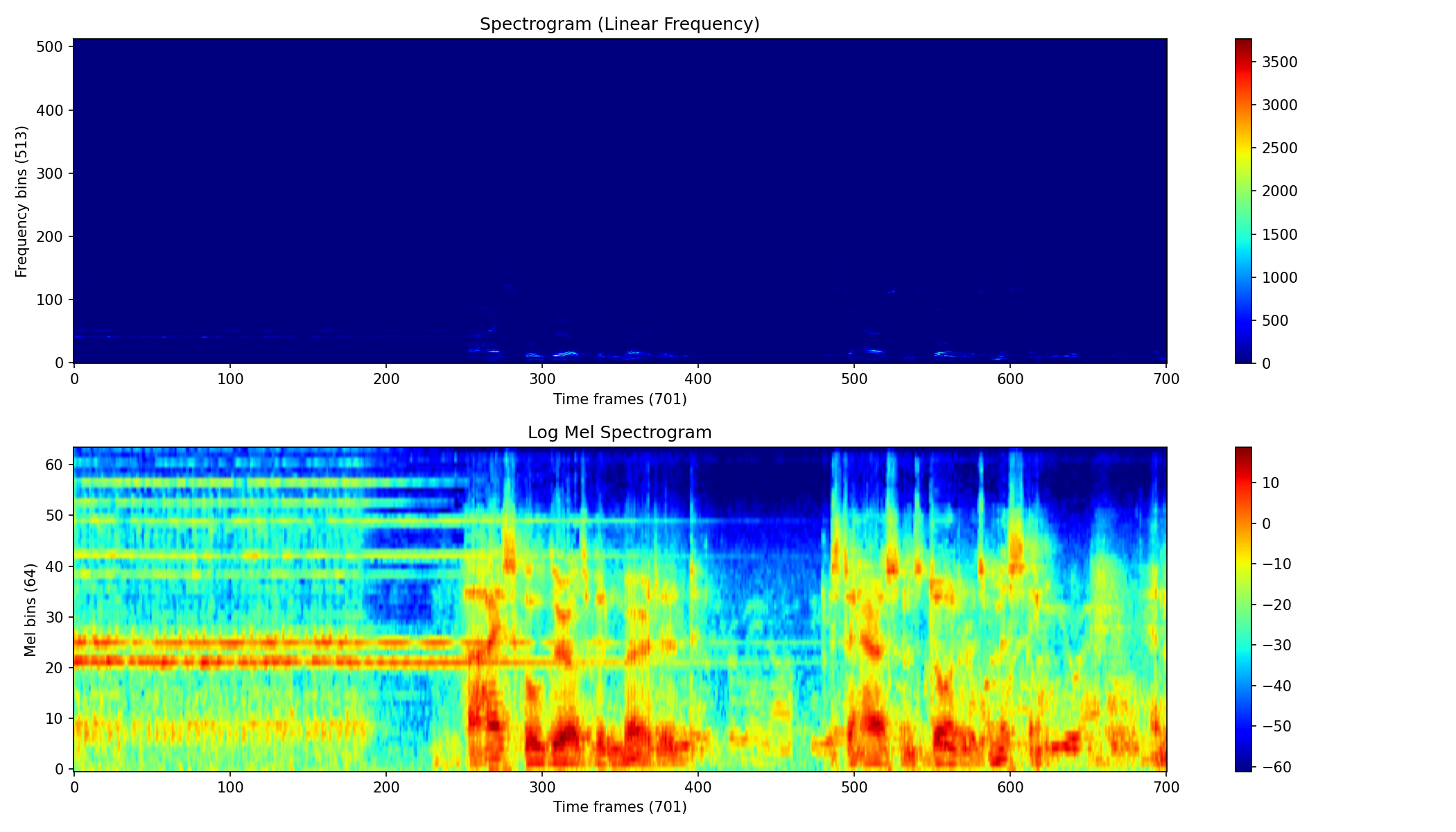
As can be seen from the spectrogram above, whether it is the linear spectrogram at the top or the Mel-scale spectrogram at the bottom, their horizontal coordinates are both the indices of the audio frames. The length of this audio file is 7 seconds, with a sampling rate of 32KHz, single channel, containing a total of 224,000 samples (7s * 32000 = 224000). The window size for FFT spectrum calculation is 1024 audio sampling points, and the number of samples for the audio frame interval (Hop size) is 320. Therefore, the 224,000 audio samples of the entire WAV file are ultimately split into 701 ($224000 / 320 + 1 = 701$) overlapping audio frames. Consequently, the horizontal coordinates of both spectrograms consist of 701 consecutive audio frames.
Regarding the vertical coordinate of the linear spectrogram, because the window size for FFT spectrum calculation is 1024 audio sampling points, the 1024 frequency domain results obtained from the FFT calculation are mirror-symmetric. Therefore, the number of frequency points in the linear spectrogram is $1024 / 2 + 1 = 513$. With a sampling rate of 32K, the frequency corresponding to each frequency point is:
- Index 0: $0\text{Hz}$ (DC component)
- Index 1: $1 \cdot 32000 / 1024 \approx 31.25\text{Hz}$
- Index 2: $2 \cdot 32000 / 1024 \approx 62.5\text{Hz}$
- …
- Index 512: $512 \cdot 32000 / 1024 = 16000\text{Hz}$
The Mel spectrogram is generated on the basis of the linear spectrogram. In the code, the mel_bins parameter sets the number of Mel filter banks to 64. By filtering and aggregating the energy of various frequency bands of the linear spectrogram in a manner that is dense at low frequencies and sparse at high frequencies, 64 energy density distributions ranging from low to high frequencies are ultimately formed on the vertical coordinate of the Mel-scale spectrogram.