A Detailed Explanation of the Calculation Workflow for Dilated Convolution and Deformable Convolution
- 25 Mar, 2026
The calculation workflow of standard convolution kernels in convolutional neural networks has been comprehensively summarized in the article A Detailed Explanation of Convolution and Pooling Calculations in Convolutional Neural Networks. This article focuses on two relatively specialized convolution operations: Dilated Convolution and Deformable Convolution.
Dilated Convolution
Simply put, compared to standard convolution, dilated convolution can forcefully expand the receptive field of the convolution operation without increasing the number of parameters.
In standard convolution calculations, the elements of the convolution kernel are adjacent to each other:
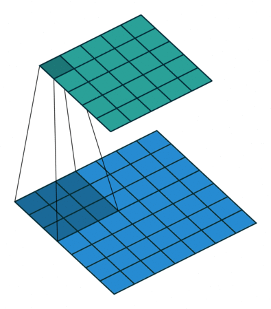
When performing dilated convolution, holes are inserted between the weight elements of the convolution kernel (i.e., padding with zeros, which are skipped during actual computation). As shown in the animation below, for a 3x3 dilated convolution, holes are inserted between each element during computation. This makes the receptive field equivalent to that of a 5x5 convolution, while the number of parameters and computational cost remain at the 3x3 level.
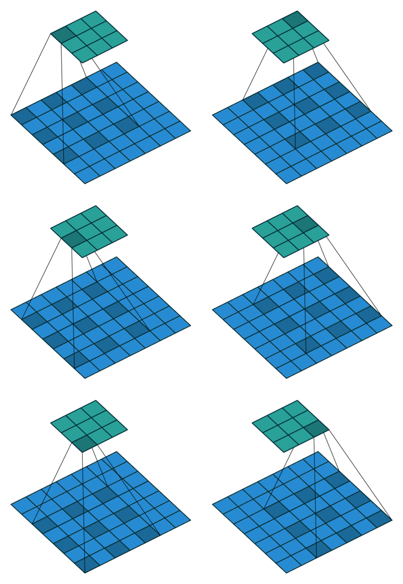
The core parameter for dilated convolution shown in the figure above is the Dilation Rate. It specifies the number of holes to be inserted between two consecutive weight elements during the convolution calculation, which represents the spacing between elements:
- d=1: Standard convolution.
- d=2: Skips one pixel between every two weight elements, and so on.
In the dilated convolution calculation workflow illustrated above, a certain number of pixels are skipped between sampling points during computation, determined by the dilation rate parameter.
Assume the input feature map is $x$ and the 2D convolution kernel is $w$, with a size of $k \times k$. For a value $y(i, j)$ at position $(i, j)$ on the output feature map, the formula for dilated convolution is:
$$ y(i, j) = \sum_{m=0}^{k-1} \sum_{n=0}^{k-1} x(i + d \cdot m, j + d \cdot n) \cdot w(m, n) $$
- Here, $d \cdot m$ and $d \cdot n$ represent the dilation effect, altering the indexing step size when reading the input $x$. When $d=1$, the above formula reduces to the standard convolution calculation formula.
- It is important to note that the number of parameters in the convolution kernel $w$ remains $k \times k$, and no extra weight parameters are added due to the dilation.
In PyTorch, nn.Conv2d already integrates the dilation parameter to specify the dilation rate during convolution.
import torch
import torch.nn as nn

# Define a dilated convolution layer
# in_channels=1, out_channels=1, kernel_size=3, stride=1, padding=2 (to keep input and output dimensions consistent), dilation=2
dilated_conv = nn.Conv2d(in_channels=1,
                         out_channels=1,
                         kernel_size=3,
                         stride=1,
                         padding=2,
                         dilation=2) # Key parameter for dilated convolution; set dilation=1 for standard convolution.
Deformable Convolution
In traditional convolutions (including dilated convolutions), regardless of the object’s shape outline, or how it is rotated, scaled, or deformed, the sampling shape of the convolution kernel is always a fixed square (e.g., 3x3, 5x5, etc.).
The theory of deformable convolution argues that: convolution kernels should possess shape-sensing and adaptive capabilities. In other words, the sampling points of the convolution kernel should not be restricted to a fixed square; instead, they should be offset according to the actual outline and size of the object. By allowing the network to learn this offset itself, precise customization of the receptive field is achieved.
The formula for deformable convolution is as follows:
$$ y(p_0) = \sum_{p_n \in \mathcal{R}} w(p_n) \cdot x(p_0 + p_n + \Delta p_n) $$
The figure below illustrates the calculation workflow of deformable convolution:
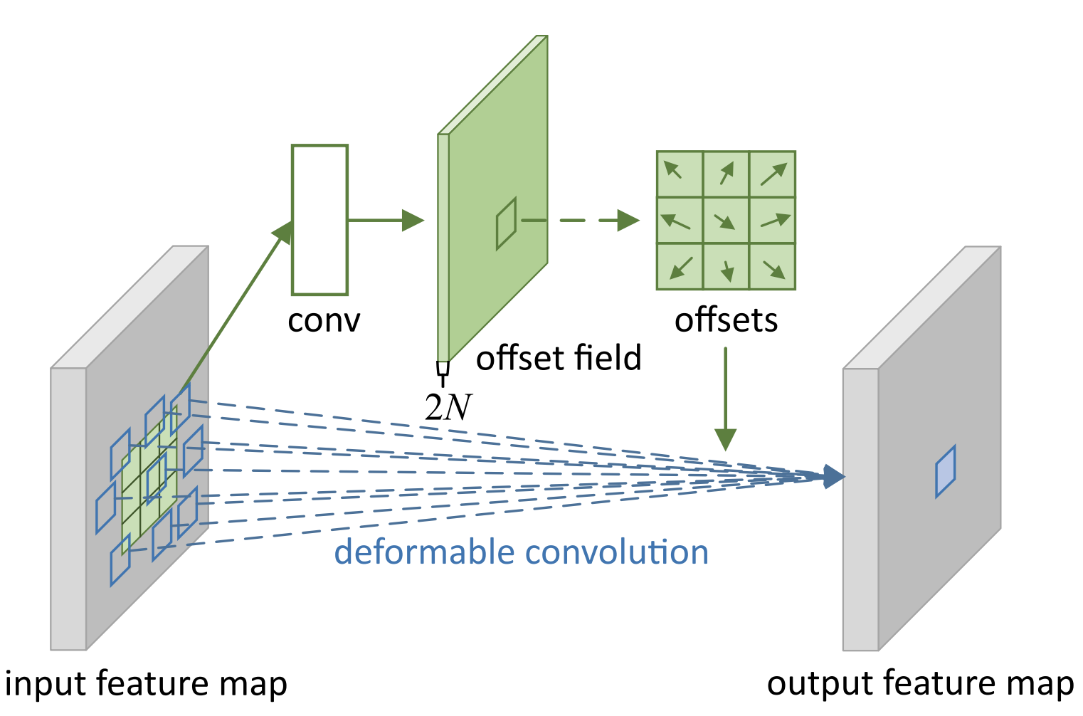
Generally speaking, the calculation of deformable convolution is divided into two stages: the first stage is responsible for generating offsets, and the second stage performs the deformable convolution calculation based on these offsets.
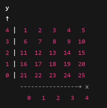
Let’s explain the calculation workflow of the above two stages using a practical example. Assume the input is a 5x5 resolution feature map, and we want to perform a 3x3 deformable convolution. We focus on the center coordinate position $(2, 2)$ of the input feature map below, which is the coordinate point with a value of 13:
Step 1: Offset Generation
The calculation in Stage 1 is relatively simple. It is essentially a standard 3x3 convolution. In this case, the output channels must be 18, because the purpose of Stage 1 is to generate two offsets ($dx, dy$) for every pixel point in the input feature map. For a 3x3 convolution, the corresponding number of output channels is $3 \times 3 \times 2 = 18$.
- Note that this offset calculation involves a separate offset convolution kernel.
Therefore, the final output of the offset calculation process is an offset tensor with the same resolution as the input feature map and 18 channels. For the feature point at position $(2, 2)$, this offset tensor contains 18 offset values:
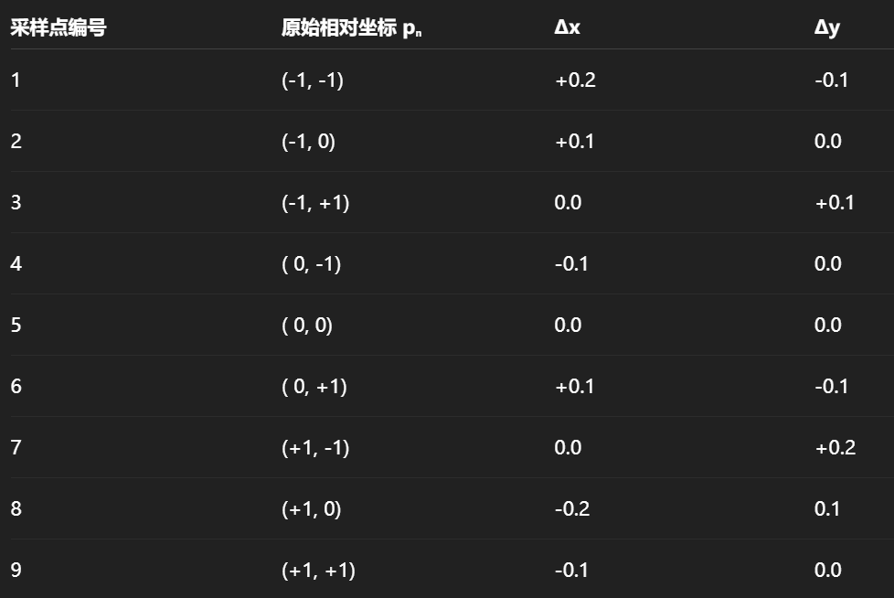
Thus, for the convolution calculation at the center point $(2, 2)$, the positions of the 9 surrounding pixels (including itself) correspond to 9 sets of $(dx, dy)$ offsets.
Step 2: Deformable Sampling
Let’s take the bottom-left point $(-1, -1)$ of the 3x3 region around position $(2, 2)$ to explain the deformable sampling workflow. According to the deformable convolution formula above:
$$ (p_0 + p_n + \Delta p_n) $$
The bottom-left point corresponds to $(dx, dy) = (0.2, -0.1)$. Plugging this into the formula gives $(2, 2) + (-1, -1) + (0.2, -0.1) = (1.2, 0.9)$. This is a non-integer coordinate (represented by the blue dot in the figure below). We find the four surrounding pixel points on the input feature map (represented by the red box in the figure below):
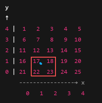
Next, bilinear interpolation is performed. The closer the distance, the higher the weight. The interpolation weights are $dx = 0.2, dy = 0.9$ (i.e., keeping only the fractional part by removing the integer part). The bilinear interpolation calculation is as follows:
$$ v = (1-dx)(1-dy) \cdot 17 + dx(1-dy) \cdot 18 + (1-dx)dy \cdot 22 + dx \cdot dy \cdot 23 = 20.476 $$
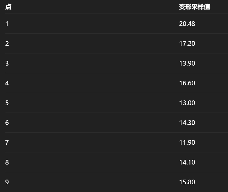
This value of 20.476 is merely the deformable convolution calculation result for the bottom-left point $(-1, -1)$. Following the exact same workflow as Step 2, perform the above calculations for all 9 positions to obtain the 9 deformed sampling values:
Step 3: Weighted Summation Using the Main Convolution Kernel
Finally, to obtain the final deformable convolution calculation result for position $(2, 2)$, element-wise multiplication is performed between the 9 values obtained above and the weight parameters of the main convolution kernel:
$$ Output(2, 2) = \sum_{n=1}^{9} x_{sampled, n} \cdot w_n $$
- $x_{sampled, n}$ represents the 9 deformed sampling values obtained in Step 2 above, and $w_n$ represents the weight parameters of the main convolution kernel.
Steps 1 through 3 above only calculate the deformable convolution result for the center position $(2, 2)$ of the input feature map. All other pixels must also go through the complete workflow of Steps 1 to 3 to obtain the deformable convolution result for the entire input feature map. As can be seen, the computational overhead of deformable convolution is significantly higher than that of standard convolution.
PyTorch does not provide a native implementation of deformable convolution, but torchvision.ops provides DeformConv2d to implement deformable convolution calculations.
import torch
from torchvision.ops import DeformConv2d

# Assume an input tensor
input_tensor = torch.randn(1, 64, 28, 28) # [B, C, H, W]

# 1. Define the convolution layer for generating offsets
# Output channels must be 2 * kernel_h * kernel_w; the following corresponds to a 3x3 convolution
offset_conv = torch.nn.Conv2d(64, 2 * 3 * 3, kernel_size=3, padding=1)
offsets = offset_conv(input_tensor)

# 2. Define the deformable convolution layer
dcn = DeformConv2d(64, 128, kernel_size=3, padding=1)

# 3. Forward pass
output = dcn(input_tensor, offsets)