Implementing a Vision Transformer (ViT) Model from Scratch

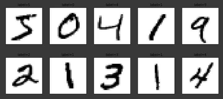
This article focuses on the task of recognizing the simple MNIST handwritten digit dataset, completing the implementation, training, and validation of a minimal Vision Transformer model to build a comprehensive understanding of the ViT implementation workflow.

The MNIST handwritten digit dataset is the simplest computer vision dataset. Implementing a Vision Transformer to recognize handwritten characters on MNIST is not overly difficult, and the data and computational requirements for model training are minimal. Therefore, training a ViT recognition model on the MNIST dataset serves as an excellent introductory experiment for learning Vision Transformers.

Regarding the overall architecture of the Vision Transformer model, you can refer to another note: [[An Introduction to the Architecture of the Vision Transformer (ViT) Model]].

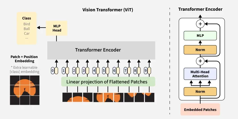
Note: Reference 1 provides a complete Vision Transformer model for recognizing the MNIST handwritten character set. This article is essentially a study record of the aforementioned material, supplemented by my own understanding of the implementation process.

As summarized in the note [[An Introduction to the Architecture of the Vision Transformer (ViT) Model]], the architecture and workflow of the ViT model can be roughly divided into the following stages: image patching, adding the Cls Token, positional encoding, the Transformer Encoder based on multi-head self-attention mechanisms, and the final classification head. Therefore, this article follows the above structure to implement a complete Vision Transformer architecture, training and testing it using the MNIST dataset.

1. Importing Necessary Packages

import torch
import torch.nn as nn
import torchvision.transforms as T
from torch.optim import Adam
from torchvision.datasets.mnist import MNIST
from torch.utils.data import DataLoader
import numpy as np

• Import torchvision.transforms to resize the MNIST character set images, ensuring the input resolution is a multiple of the patch resolution, and to convert MNIST character set image data into Tensor format.
• Use Adam, included in torch.optim, as the optimizer for the training process.
• Automatically download the MNIST dataset from the official PyTorch website using torchvision.datasets.mnist.

2. Patch Embeddings

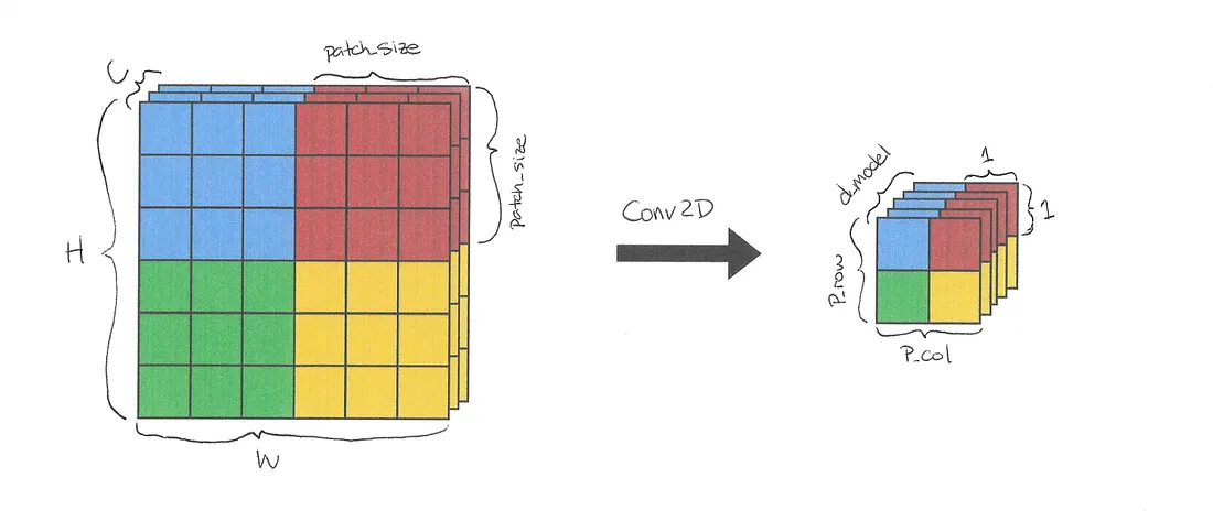
This step implements slicing the input image into fixed-size patches and serializing them. As mentioned in [[An Introduction to the Architecture of the Vision Transformer (ViT) Model]], this functionality is typically implemented using a 2D convolution (Conv2d) where the stride equals the kernel size (kernel_size).

nn.Conv2d(self.n_channels, self.d_model, kernel_size=self.patch_size, stride=self.patch_size)

The Conv2d operation above is actually a convolutional projection:

• kernel_size=patch_size: Extracts each patch using a patch_size × patch_size kernel.
• stride=patch_size: Sets the stride equal to the patch size, achieving non-overlapping slicing.
• Output channels = d_model: Maps each patch into a d_model-dimensional vector, vectorizing each patch.

The complete code for patch embedding is as follows:

class PatchEmbedding(nn.Module):
    def __init__(self, d_model, img_size, patch_size, n_channels):
        super().__init__()

        self.d_model = d_model # Dimension length of each patch after vectorization
        self.img_size = img_size # Input image resolution
        self.patch_size = patch_size # Resolution of each patch
        self.n_channels = n_channels # Number of input image channels

        self.linear_project = nn.Conv2d(self.n_channels, self.d_model, kernel_size=self.patch_size, stride=self.patch_size)

    # B: Batch size
    # C: Number of input image channels
    # H: Input image height
    # W: Input image width
    # P_col: Number of patch columns
    # P_row: Number of patch rows
    # P: Total number of patches, P_col * P_row
    def forward(self, x):
        x = self.linear_project(x) # (B, C, H, W) -> (B, d_model, P_col, P_row)
        x = x.flatten(2) # (B, d_model, P_col, P_row) -> (B, d_model, P)
        x = x.transpose(1, 2) # (B, d_model, P) -> (B, P, d_model)
        return x

In the forward operation above, self.linear_project(x) converts the dimensions of an input image from (C, H, W) to (d_model, P_col, P_row);

x.flatten(2) flattens all patches, yielding $P$ serialized patches, each with a dimension length of d_model. This is effectively the output result of the patch embedding operation;

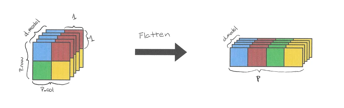
The final x = x.transpose operation simply swaps the output data dimensions to fit the standard input format of the Transformer architecture.

3. Cls Token and Positional Encoding

The logic for prepending a Cls Token to the patch list of each image in a batch is relatively simple: create a new cls token with a length equal to the patch vector, and place this token at the very beginning of the patch vectors as the 0-th token.

In addition to the Cls Token, positional encodings must be added to the patch vectors. Each positional encoding is unique to the position it represents, enabling the model to recognize the location of each patch. To add positional encodings to the patch vectors, they must share the same dimension, d_model. The formula for constructing the position vectors is as follows:

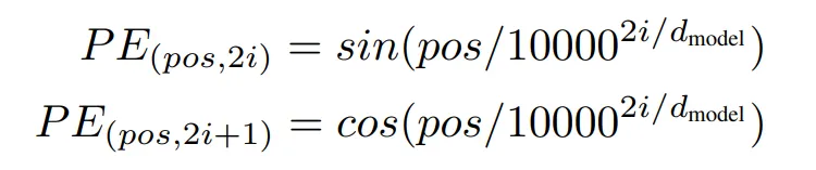
Thus, broadly speaking, this step consists of two operations: prepending a Cls token to the patch vector list for each sample image in the batch, and adding positional encodings to all vectors. The complete code is as follows:

class PositionalEncoding(nn.Module):
    def __init__(self, d_model, max_seq_length):
        super().__init__()
        self.cls_token = nn.Parameter(torch.randn(1, 1, d_model)) # Create a new Cls Token of length d_model

        # Construct positional encodings according to the formula above
        pe = torch.zeros(max_seq_length, d_model)
        for pos in range(max_seq_length):
            for i in range(d_model):
                if i % 2 == 0:
                    pe[pos][i] = np.sin(pos/(10000 ** (i/d_model)))
                else:
                    pe[pos][i] = np.cos(pos/(10000 ** ((i-1)/d_model)))
        self.register_buffer('pe', pe.unsqueeze(0))

    def forward(self, x):
        # Add Cls Token for each sample image
        tokens_batch = self.cls_token.expand(x.size()[0], -1, -1)
        # Concatenate Cls Token and Patch Embedding
        x = torch.cat((tokens_batch,x), dim=1)
        # Add positional encoding
        x = x + self.pe

        return x

4. Implementation of Single-Head and Multi-Head Attention Modules

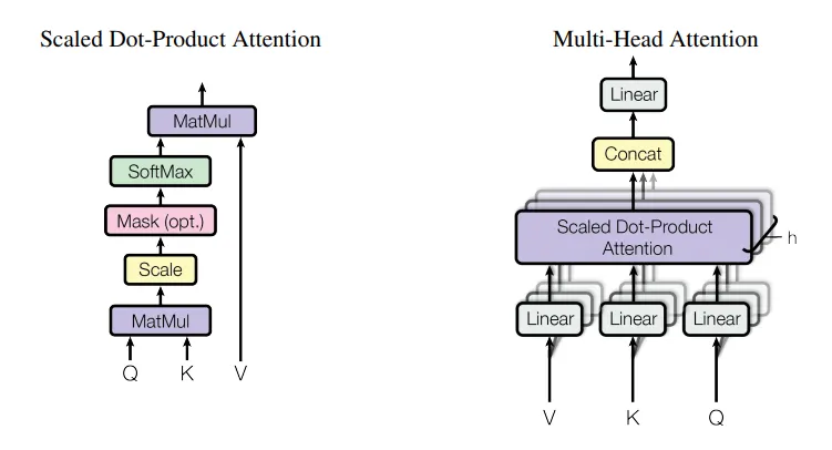
The theory and calculation workflow of multi-head attention modules have already been thoroughly summarized and explained in the article [[How to Understand the Multi-Head Attention Mechanism in the Transformer Architecture?]], and will not be repeated here.

The calculation formula for the single-head attention mechanism is as follows:

$$ \text{Attention}(Q, K, V) = \text{softmax}\left(\frac{QK^T}{\sqrt{d_k}}\right)V $$

You can combine the formula above with the comments in the code to understand the calculation logic and workflow of single-head attention, which is essentially a step-by-step implementation of the formula:

class AttentionHead(nn.Module):
    def __init__(self, d_model, head_size):
        super().__init__()
        self.head_size = head_size # Dimension length of each attention head

        # Initialize linear transformation layers for Q, K, V
        self.query = nn.Linear(d_model, head_size)
        self.key = nn.Linear(d_model, head_size)
        self.value = nn.Linear(d_model, head_size)

    def forward(self, x):
        # Calculate Q, K, V vectors for the input data
        Q = self.query(x)
        K = self.key(x)
        V = self.value(x)

        # Calculate dot-product attention scores for Q and K
        attention = Q @ K.transpose(-2,-1)

        # Scaling
        attention = attention / (self.head_size ** 0.5)
        attention = torch.softmax(attention, dim=-1)
        attention = attention @ V

        return attention

Based on the single-head attention module above, implementing the multi-head attention module is relatively straightforward: compute multiple attention heads independently, concatenate their results, and finally pass them through a linear layer to further fuse and output the features from all single-head outputs:

class MultiHeadAttention(nn.Module):
    def __init__(self, d_model, n_heads):
        super().__init__()

        self.head_size = d_model // n_heads # Calculate dimension length for each attention head
        self.W_o = nn.Linear(d_model, d_model)
        self.heads = nn.ModuleList([AttentionHead(d_model, self.head_size) for _ in range(n_heads)])

    def forward(self, x):
        # Compute each attention head independently and concatenate the results
        out = torch.cat([head(x) for head in self.heads], dim=-1)

        out = self.W_o(out)
        return out

The workflow and structure of the single-head and multi-head attention modules are illustrated below:

5. Transformer Encoder

Next is the implementation of the complete Transformer Encoder. The structure of the Transformer Encoder is shown below:

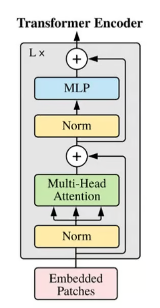
Its corresponding code is:

class TransformerEncoder(nn.Module):
    def __init__(self, d_model, n_heads, r_mlp=4):
        super().__init__()
        self.d_model = d_model
        self.n_heads = n_heads

        # Normalization layer 1
        self.ln1 = nn.LayerNorm(d_model)

        # Multi-head attention layer
        self.mha = MultiHeadAttention(d_model, n_heads)

        # Normalization layer 2
        self.ln2 = nn.LayerNorm(d_model)

        # MLP feed-forward neural network layer
        self.mlp = nn.Sequential(
            nn.Linear(d_model, d_model*r_mlp),
            nn.GELU(),
            nn.Linear(d_model*r_mlp, d_model)
        )

    def forward(self, x):
        # Residual connection between normalization layer 1 and multi-head attention layer output
        out = x + self.mha(self.ln1(x))
        # Residual connection between normalization layer 2 and MLP feed-forward network output
        out = out + self.mlp(self.ln2(out))

        return out

6. The Complete Vision Transformer Model

The architecture of the fully implemented Vision Transformer model is shown below:

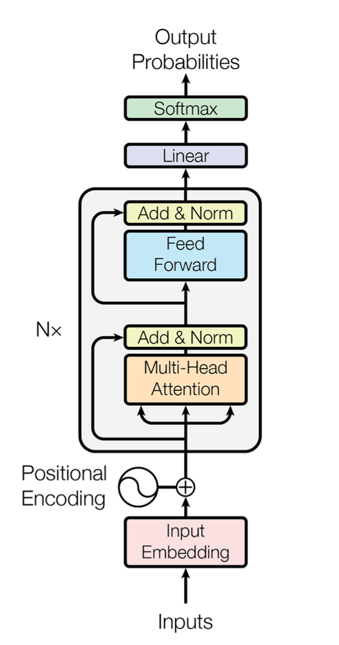
• Input images first undergo slicing, vectorization, and serialization in the PatchEmbedding module.
• The serialized patch vectors are then supplemented with an extra Cls Token and position vectors in the PositionalEncoding module.
• This data is then processed through $N$ consecutive TransformerEncoder modules, repeatedly extracting and fusing image features via multi-head attention modules.
• Finally, it passes through a classification head and outputs classification probabilities via Softmax.

The complete implementation of the Vision Transformer model is as follows:

class VisionTransformer(nn.Module):
    def __init__(self, d_model, n_classes, img_size, patch_size, n_channels, n_heads, n_layers):
        super().__init__()

        # Input image resolution must be divisible by patch_size, and patch vector length must be divisible by attention module dimension length
        assert img_size[0] % patch_size[0] == 0 and img_size[1] % patch_size[1] == 0, "img_size dimensions must be divisible by patch_size dimensions"
        assert d_model % n_heads == 0, "d_model must be divisible by n_heads"

        self.d_model = d_model # Dimension length of each patch vector in the model
        self.n_classes = n_classes # Number of classes for classification task, corresponding to digits 0-9
        self.img_size = img_size # Input image resolution
        self.patch_size = patch_size # Resolution of each patch
        self.n_channels = n_channels # Number of input image channels, MNIST dataset is grayscale with 1 channel
        self.n_heads = n_heads # Number of attention heads

        # Calculate how many patches the input image can be split into
        self.n_patches = (self.img_size[0] * self.img_size[1]) // (self.patch_size[0] * self.patch_size[1])
        self.max_seq_length = self.n_patches + 1 # Maximum sequence length, including the Cls Token

        self.patch_embedding = PatchEmbedding(self.d_model, self.img_size, self.patch_size, self.n_channels)
        self.positional_encoding = PositionalEncoding( self.d_model, self.max_seq_length)
        self.transformer_encoder = nn.Sequential(*[TransformerEncoder( self.d_model, self.n_heads) for _ in range(n_layers)])

        # Classification MLP
        self.classifier = nn.Sequential(
            nn.Linear(self.d_model, self.n_classes),
            nn.Softmax(dim=-1)
        )

    def forward(self, images):
        x = self.patch_embedding(images)
        x = self.positional_encoding(x)
        x = self.transformer_encoder(x)
        x = self.classifier(x[:,0])

        return x

7. Training and Testing

Finally, train the model constructed above, and validate the trained model using the MNIST test dataset.

Hyperparameter Settings

The hyperparameter settings for training the model are as follows:

# Hyperparameters
d_model = 9  # Dimension length of each patch vector
n_classes = 10  # Number of classes for classification task, corresponding to digits 0-9
img_size = (32,32)  # Input image resolution
patch_size = (16,16)  # Resolution of each patch
n_channels = 1  # Number of input image channels, MNIST is grayscale with 1 channel
n_heads = 3  # Number of attention heads
n_layers = 3  # Number of Transformer Encoder layers
batch_size = 128  # Number of samples per batch
epochs = 15  # Number of training epochs
alpha = 0.005  # Learning rate

Preparation of Training and Testing Datasets

Training and testing use the MNIST dataset downloaded from the official PyTorch website. Use the following code to download the dataset and prepare the dataloaders:

transform = T.Compose([
    T.Resize(img_size),
    T.ToTensor()
])

train_set = MNIST(
    root="datasets", train=True, download=True, transform=transform
)
test_set = MNIST(
    root="datasets", train=False, download=True, transform=transform
)

train_loader = DataLoader(train_set, shuffle=True, batch_size=batch_size)
test_loader = DataLoader(test_set, shuffle=False, batch_size=batch_size)

Model Training

Next, train the parameters of the constructed model. The entire training execution flow is largely similar to the handwritten digit recognition training process based on Convolutional Neural Networks described in the article [[[Implementing Handwritten Digit Recognition with Convolutional Neural Networks Based on PyTorch]]]:

device = torch.device("cuda" if torch.cuda.is_available() else "cpu")
print("Using device: ", device, f"({torch.cuda.get_device_name(device)})" if torch.cuda.is_available() else "")

transformer = VisionTransformer(d_model, n_classes, img_size, patch_size, n_channels, n_heads, n_layers).to(device)
optimizer = Adam(transformer.parameters(), lr=alpha) # Adam optimizer with learning rate alpha
criterion = nn.CrossEntropyLoss() # Cross-entropy loss function

for epoch in range(epochs):
    training_loss = 0.0

    for i, data in enumerate(train_loader, 0):
        inputs, labels = data
        inputs, labels = inputs.to(device), labels.to(device)
        optimizer.zero_grad()
        outputs = transformer(inputs)
        loss = criterion(outputs, labels)
        loss.backward()
        optimizer.step()
        training_loss += loss.item()

    print(f'Epoch {epoch + 1}/{epochs} loss: {training_loss  / len(train_loader) :.3f}')

After training for 15 epochs, the printed loss values show that the loss converges steadily downward:

Using device:  cuda (NVIDIA GeForce RTX 5070 Ti Laptop GPU)
Epoch 1/15 loss: 1.707
Epoch 2/15 loss: 1.569
Epoch 2/15 loss: 1.569
Epoch 3/15 loss: 1.556
...
Epoch 13/15 loss: 1.524
Epoch 14/15 loss: 1.524
Epoch 15/15 loss: 1.522

Model Testing

Finally, use the trained model above to test on the MNIST test dataset:

correct = 0
total = 0

with torch.no_grad():
    for data in test_loader:
        images, labels = data
        images, labels = images.to(device), labels.to(device)
        outputs = transformer(images)
        _, predicted = torch.max(outputs.data, 1)
        total += labels.size(0)
        correct += (predicted == labels).sum().item()
    print(f'\nModel Accuracy: {100 * correct // total} %')

After the aforementioned 15 rounds of testing, the test accuracy of the model on the test set reached 93%.

References

• Building a Vision Transformer Model From Scratch | by Matt Nguyen | Toward Humanoids | Medium

---

Attempting to understand and explain technical problems from the perspective of underlying principles: Audio/Video / Cameras / Smart Home / Bluetooth / WiFi / Wireless Communication / AI.

Please follow the WeChat Official Account: Pavel Han.