Background Knowledge Summary of the YOLOv5 Loss Function
- 10 Feb, 2026
Based on versions v6.0/v6.1 of the YOLOv5 model, this article provides a detailed summary and explanation of the loss function calculation workflow and the background knowledge involved in its code implementation.
As shown in the structure of the YOLOv5 detection head below, similar to previous generations, the bounding box data output by each grid in the YOLOv5 model contains 5 + NC information divided into three parts: the coordinate positions of the predicted bounding box, the detection confidence, and the class probabilities.
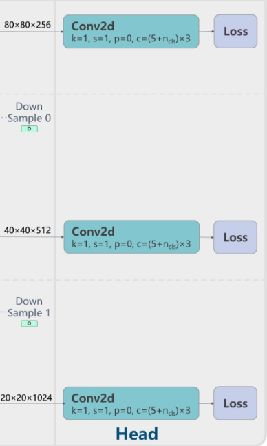
Accordingly, the loss function consists of three components:
- Bounding box regression loss (Box Loss)
- Object confidence loss (Obj Loss)
- Classification loss (Cls Loss)
Among them, the bounding box regression loss uses CIoU (Complete IoU) loss, while both the object confidence loss and the classification loss use Binary Cross-Entropy (BCE) loss.
Binary Cross-Entropy (BCE)
First, let’s explain the calculation workflow of BCE using the simplest binary classification problem. Assuming the ground truth label of the training data is $y$ (0 or 1), and the model’s prediction is $p$ (a probability value between 0 and 1), the formula for the BCE loss function is:
$$ BCE(y,p)=−[y⋅log(p)+(1−y)⋅log(1−p)] $$
Because taking the logarithm of a decimal between 0 and 1 always yields a result less than 0, the output of the BCE formula above is always positive. For $\log(x)$, when $x=1$, $\log(x)=0$; when $x$ is between 0 and 1, $\log(x)$ is negative and decreases as $x$ approaches 0; when $x$ approaches 0, $\log(x)$ tends toward negative infinity.
Therefore:
- When the label $y=1$, the loss function simplifies to $-log(p)$. In this case, the higher the predicted probability $p$, the smaller the loss value, getting closer to 0.
- When the label $y=0$, the loss simplifies to $-log(1-p)$. In this case, the lower the predicted probability $p$, the smaller the loss value, getting closer to 0.
As shown above, the predicted value $p$ used in cross-entropy calculation should be between 0 and 1. Therefore, for the logits output by the three detection heads of the YOLOv5 model, a sigmoid function is applied to the logits before computing the BCE loss. In fact, the YOLOv5 source code uses the BCEWithLogitsLoss function for both object confidence loss and classification loss:
BCEcls = nn.BCEWithLogitsLoss(pos_weight=torch.tensor([h["cls_pw"]], device=device))
BCEobj = nn.BCEWithLogitsLoss(pos_weight=torch.tensor([h["obj_pw"]], device=device))
The implementation of the BCEWithLogitsLoss function actually corresponds to the following formula:
$$ BCE(p,t)=−[t⋅log(σ(p))+(1−t)⋅log(1−σ(p))] $$
where $p$ is the raw logit output by the model, $\sigma$ is the sigmoid activation function, and $t$ is the target value.
Weight Control in Positive Sample Loss Calculation
It is worth noting that the BCEWithLogitsLoss function definition above passes two pos_weight parameters via hyperparameters: cls_pw and obj_pw. By default, both parameters are set to 1.0 in the hyperparameter configuration file. In this case, the loss for positive samples ($t > 0$) in the BCE formula is multiplied by $\gamma$, while the loss for negative samples ($t = 0$) remains unchanged. The actual equivalent formula becomes:
$$ BCE(p,t)=−[γ⋅t⋅log(σ(p))+(1−t)⋅log(1−σ(p))] $$
Therefore, if you need to adjust the proportion of positive sample loss during model training for class loss and confidence loss, you can tune the cls_pw and obj_pw parameters. Setting these parameters to values greater than 1.0 will strengthen the training penalty for positive samples; otherwise, it will weaken it.
- For example, if a high miss rate or lower prediction confidence for positive samples is observed during training, you can try setting
obj_pw > 1.0(e.g., $1.5 \sim 5.0$) to strengthen the positive sample penalty. Conversely, if there are too many false positives (i.e., background incorrectly predicted as positive samples), you can slightly decreaseobj_pw($<1.0$).
Construction of the Positive Sample List for Loss Calculation
As summarized in the article YOLOv5 Model Prediction Output and Its NMS Algorithm Analysis, YOLOv5 outputs over 20,000 prediction boxes for a single image during inference, the vast majority of which are invalid. To compute the loss during training, we must first find a list of positive samples that closely match the ground truth boxes from these 20,000+ output prediction boxes. This is precisely what the build_targets function does in the YOLOv5 loss calculation code.
In summary: The build_targets function is responsible for matching the ground truth boxes of training samples with the model’s anchors, thereby filtering out the anchor positions from the model’s output tensors that are responsible for detecting specific ground truth boxes. These matched anchor positions serve as positive samples, which are subsequently used to compute the Box Loss, Objectness Loss, and Class Loss. Negative samples (i.e., background) retain a default object confidence value of 0.
The construction of the positive sample list can be divided into three steps: anchor matching, grid assignment with neighborhood expansion, and positive sample list generation.
Anchor Matching
For each ground truth box labeled in the training samples, YOLOv5 uses a shape-matching logic to find suitable positive prediction samples from the prediction boxes output by the three detection layers: for the output of any detection layer, as long as the anchor’s shape (i.e., aspect ratio) does not differ too much from the ground truth (GT) shape, that anchor can be used to predict that GT. As a result, a single GT box can be predicted by anchors of multiple scales simultaneously (as long as the shape meets the detection criteria).
Specifically for each detection layer, the width and height configurations of the anchor boxes for each level are pre-defined via the anchors parameter in the model configuration file. Each grid cell in every detection layer utilizes three anchor boxes to detect objects in the image according to the aspect ratios listed in the table below:
anchors:
  - [10, 13, 16, 30, 33, 23] # P3/8
  - [30, 61, 62, 45, 59, 119] # P4/16
  - [116, 90, 156, 198, 373, 326] # P5/32
This step processes the three prediction feature layers (P3, P4, and P5) independently. For each GT box, the system calculates its width and height matching status against the three pre-defined anchors on the current feature layer using the following logic.
Assuming $w_{gt}, h_{gt}$ are the width and height of the GT box, and $w_{anchor}, h_{anchor}$ are the width and height of the anchor, the ratios $r_w$ and $r_h$ are calculated using the following formulas:
$$ \begin{gather} r_w = w_{gt} / w_{anchor} \ r_h = h_{gt} / h_{anchor} \end{gather} $$
To determine whether the shapes match, the following condition is checked, where anchor_t is a hyperparameter with a default value of 4.0:
$$ \max(r_w, 1/r_w, r_h, 1/r_h) < \text{anchor_t} $$
The implication of this ground truth-to-anchor matching condition is: if the side length of the GT is between 1/4 and 4 times the side length of the anchor, we consider the anchor to “resemble” the GT, making it a potential match. Otherwise, the anchor is discarded and treated as negative background.
Grid Assignment and Neighborhood Expansion
After determining which anchor shapes are suitable using the logic above, the next step is to determine which grid cell on the feature map of that layer is responsible for prediction. First, the center point of the GT box is located by calculating its coordinates $(g_x, g_y)$ on the current feature map. Then, taking the floor of these coordinates yields the grid coordinates $(i, j)$ where the GT center resides: $i = \lfloor g_x \rfloor, j = \lfloor g_y \rfloor$.
Additionally, beyond the grid determined by center localization alone, YOLOv5 incorporates a key innovation known as cross-grid neighborhood expansion. That is, after locating the feature map grid containing the GT center, YOLOv5 not only designates this grid as a positive sample, but also includes the four nearest neighboring grid cells (directly above, below, left, and right of the center grid) as positive sample candidates. Which adjacent grids are ultimately selected as positive samples depends on the offset position of the center point within the grid. For example, if the center point is located in the top-left corner of the grid, the current grid + left neighbor + top neighbor will be output as positive samples corresponding to that GT; if the center point is located in the bottom-right corner, the current grid + right neighbor + bottom neighbor will be output.
Therefore, generally speaking, if an anchor box’s aspect ratio matches a GT box on a specific detection layer, the system will generate 3 positive prediction boxes for that GT box on that layer. Similarly, if a GT box finds two anchor boxes matching its aspect ratio on the current detection layer, the system will generate 6 positive prediction boxes for that GT box on that layer.
Generation of the Positive Sample List
By performing matching and expansion for each GT box across all three detection layers using the logic above, the complete positive sample list is finally obtained. The build_targets function ultimately outputs the following four parameters for subsequent loss calculation:
tcls: Contains the class indices of the ground truth boxes corresponding to all positive samples.tbox: Contains the bounding box coordinate information of the ground truth boxes corresponding to all positive samples.indices: Provides the indices of all positive samples within the model prediction tensorpi, used to precisely extract positive sample predictions frompi(which has a shape of[bs, na, grid_h, grid_w, 5+nc]).anch: Contains the widths and heights of the matching anchors corresponding to all positive samples.
As we can see, for an input image of size $640 \times 640$, the model’s three detection layers output a total of over 20,000 anchors per image during inference. However, even after the neighborhood expansion described above, the final generated positive samples typically number only a dozen or a few tens. In other words, positive samples account for approximately $0.1% \sim 0.2%$, while negative samples (background) account for over $99.8%$. This is the severe class imbalance problem that all object detection models must face.
The Sample Imbalance Problem and Countermeasures
To address issues such as the aforementioned positive-negative sample imbalance, training class imbalance, and easy-hard sample imbalance, the YOLOv5 model provides multiple mechanisms.
Negative Samples Participate Only in Confidence Loss Calculation
As mentioned above, the YOLOv5 loss function consists of three parts: Box Loss (localization), Cls Loss (classification), and Obj Loss (confidence). The total loss is a weighted sum of these three components.
Not all loss functions are affected by negative samples during the loss calculation. Box Loss and Cls Loss are computed exclusively using positive samples! Those 20,000+ negative samples (i.e., background) do not participate in coordinate regression or class classification loss calculations at all. The effect is that, regardless of how many negative samples there are, they do not interfere with the model learning “where the object is” and “what the object is.” Objectness Loss is the only loss component in which both positive and negative samples participate. For negative samples, the target object confidence is 0, while for positive samples, the target is the CIoU value (typically between 0 and 1). Therefore, it is only in the confidence calculation that we need to combat positive-negative sample imbalance.
”Soft Labeling” of Positive Samples (IoU-Awareness)
In early YOLO versions, the confidence label for all positive samples was simply 1. In YOLOv5, however, the objectness target for positive samples is set to the CIoU value between the predicted box at that location and the ground truth (GT) box:
# Regression
pxy = pxy.sigmoid() * 2 - 0.5
pwh = (pwh.sigmoid() * 2) ** 2 * anchors[i]
pbox = torch.cat((pxy, pwh), 1)  # predicted box
iou = bbox_iou(pbox, tbox[i], CIoU=True).squeeze()  # iou(prediction, target)
lbox += (1.0 - iou).mean()  # iou loss

obji = self.BCEobj(pi[..., 4], tobj)
This means that positive samples predicted more accurately (i.e., with higher IoU) contribute a more rational pulling force to the loss. This mechanism enables the model not just to distinguish between “presence or absence of an object,” but to differentiate between “high-quality objects” and “background.” To a certain extent, this also smooths out the extreme polarization between positive and negative samples.
Focal Loss
Although YOLOv5 disables Focal Loss by default (fl_gamma=0.0 in the hyperparameter file), the codebase actually integrates an implementation of Focal Loss, which can be enabled by setting the value of fl_gamma in the hyperparameter file.
The working principle of Focal Loss is that it can automatically reduce the weight of easy samples (such as boxes that are obviously background at a glance), allowing the model to focus on difficult samples. Since most background regions are very easy to distinguish (e.g., pure black areas, sky), Focal Loss can drastically reduce the loss generated by this massive volume of negative samples, thereby eliminating the impact of imbalance.
The general idea is: if the model is very confident about a sample (relatively high confidence), its loss weight is scaled down close to 0 during loss calculation; if the model lacks confidence in a sample (relatively low confidence), its loss is preserved during calculation.
In terms of specific calculation, Focal Loss multiplies the standard BCE result by a factor of $(1 - p_t)^\gamma$:
$$ FL(p_t) = -(1 - p_t)^\gamma \log(p_t) $$
Here, $\gamma$ (gamma, i.e., the value set for the fl_gamma hyperparameter) is a hyperparameter, usually set to 2.
- For easy samples, the model’s prediction output is very accurate, e.g., $p_t = 0.99$. In this case, the Focal Loss factor calculated using the formula above is: $(1 - 0.99)^2 = 0.01^2 = 0.0001$. As a result, the original loss is scaled down by 10,000 times, making almost zero contribution to the gradient.
- For difficult samples, the model’s prediction is poor, e.g., $p_t = 0.2$. Its Focal Loss factor is: $(1 - 0.2)^2 = 0.8^2 = 0.64$. Consequently, the loss is only slightly reduced while still maintaining a large value, retaining its guiding significance for the model.
Of course, in YOLOv5, Focal Loss is applied only to the calculation of Objectness Loss ($L_{obj}$) and Classification Loss ($L_{cls}$), and is not used for Box Regression Loss.