Interpretation of the YOLOv8 Model Network Architecture
- 20 Nov, 2025
This article details and summarizes the similarities and differences in network architecture design between the YOLOv8 and YOLOv5 models by comparing the two, thereby providing a comprehensive and in-depth understanding of the YOLOv8 model structure.
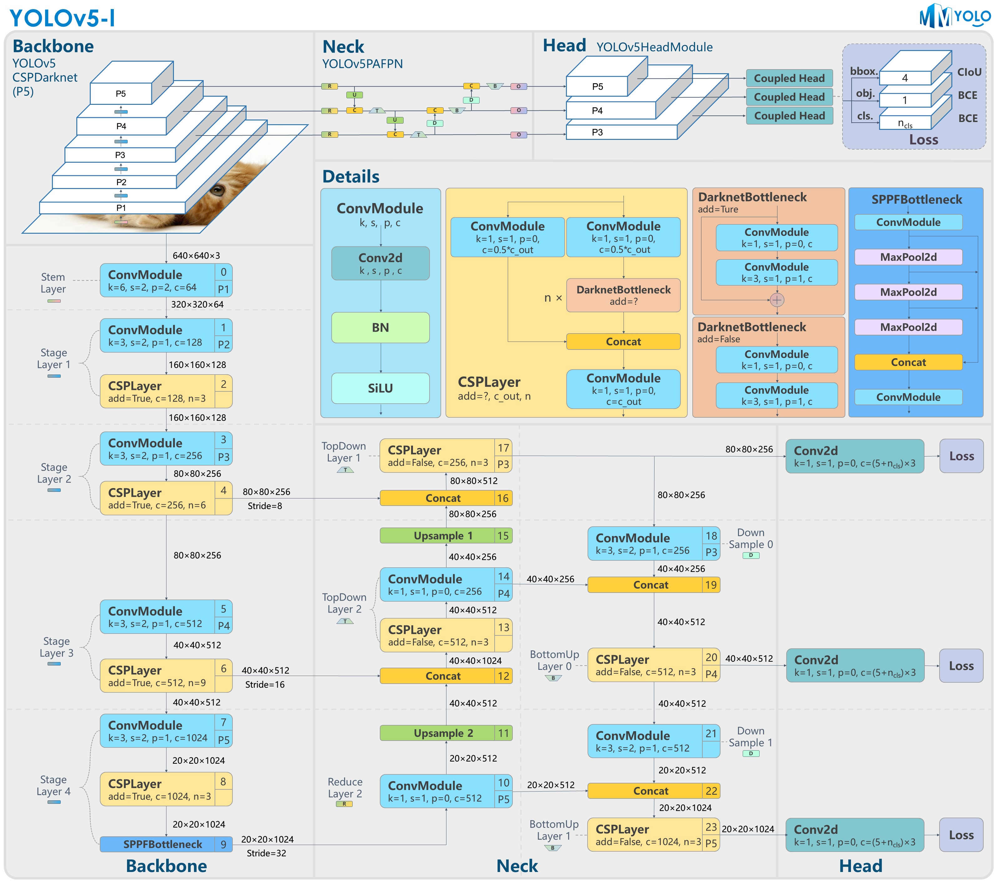
Below is the overall architecture diagram of the YOLOv5 model:
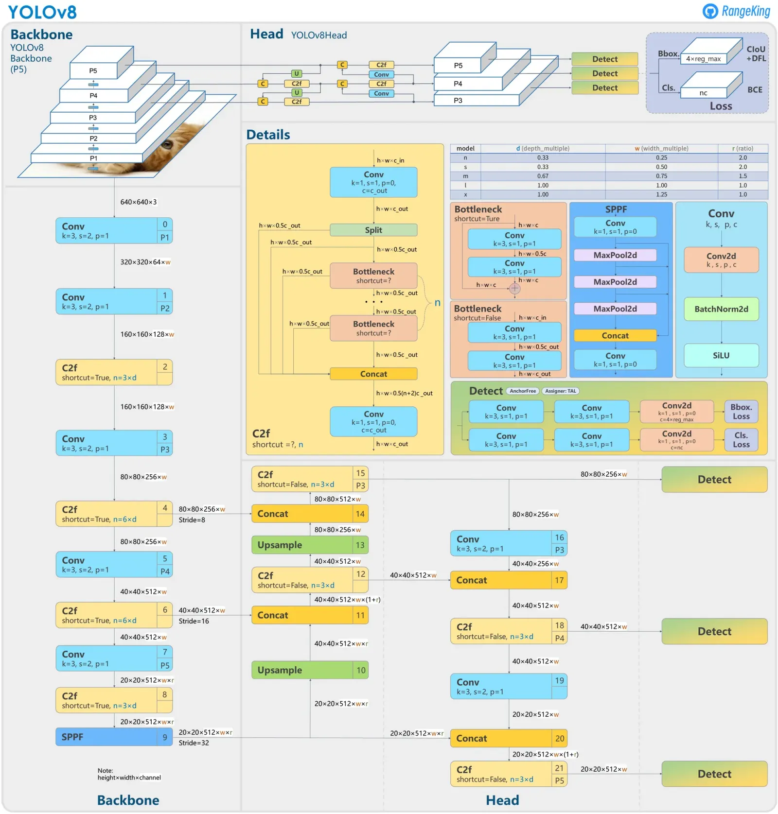
Below is the overall network architecture diagram of the YOLOv8 model:
Backbone Network
Comparing the Backbone networks on the left side of the YOLOv5 and YOLOv8 architecture diagrams above, it can be seen that the overall structures of the backbone networks of these two models are very similar. The main differences lie in the following two points:
- At the P1 layer: YOLOv5 uses either the FOCUS module (older versions) or a 6x6 convolutional layer with a stride of 2 (newer versions) to perform initial downsampling of the input image from 640x640x3 to a 320x320x64 feature map. In contrast, the YOLOv8 model uses a 3x3 convolutional layer with a stride of 2—the same as other dimension-reduction modules in the backbone—to reduce the resolution, taking the same 320x320x64 feature map as input.
- The YOLOv8 model replaces the CSPLayer module (i.e., the C3 module) of the YOLOv5 model with the C2f module, where the C2f module is one of the core innovations of YOLOv8.
C2f Module
As mentioned above, the C2f module in the YOLOv8 backbone network is one of the greatest innovations in its architectural design. First, let’s compare the structural differences between the C3 module of YOLOv5 and the C2f module of YOLOv8:
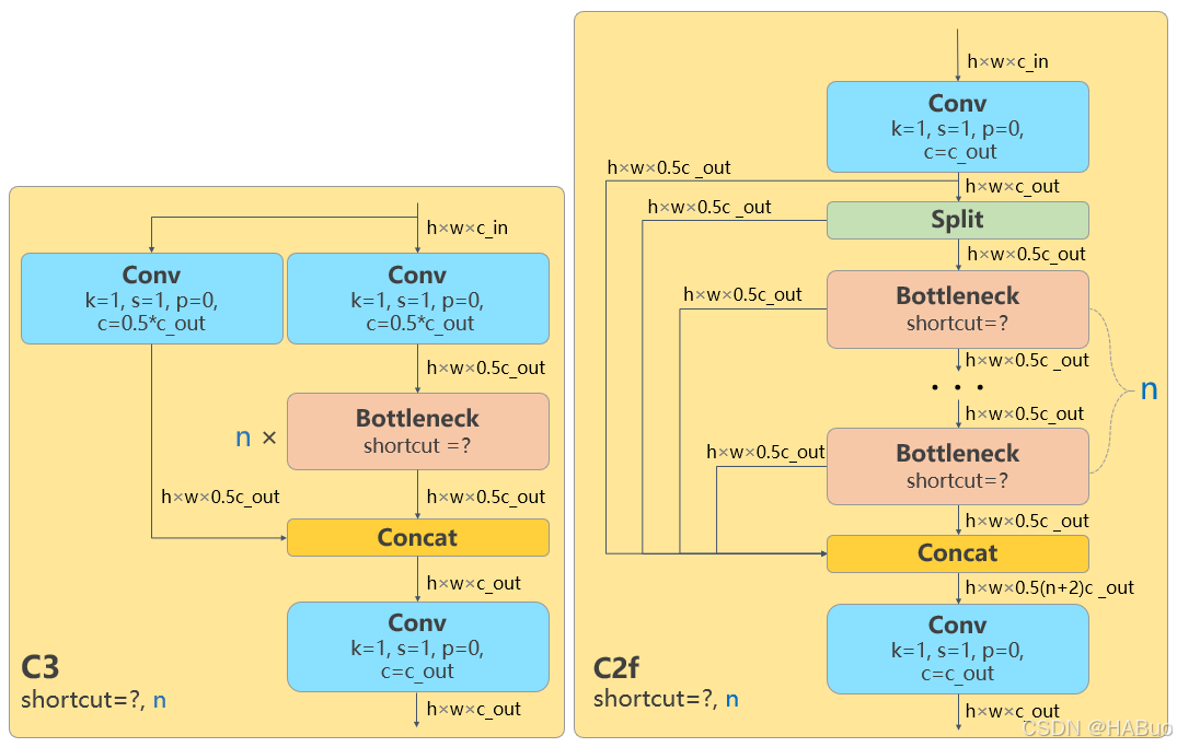
As can be seen, the C3 module adopts a dual-branch parallel structure, splitting the input feature map into two parts processed respectively by the main branch and the shortcut branch:
- Main branch: After dimensionality reduction via a 1x1 convolution, features are extracted through multiple Bottleneck residual modules (the number of residual modules can be set via the
depth_multipleparameter). - Shortcut branch: Processed directly through a 1x1 convolution to preserve the original feature information.
- Final feature fusion: The outputs of the two branches are concatenated directly along the channel dimension and then fused via a 1x1 convolution before outputting.
In contrast, the C2f module adopts a multi-stage serial structure, and its design appears somewhat more complex:
- Initial processing: The input feature map uniformly passes through a 1x1 convolution to generate intermediate feature maps.
- Feature splitting: The intermediate feature map is split into two parts; one part is processed sequentially through multiple Bottleneck modules, while the other part is passed directly to the end.
- Multi-stage processing: For a series of subsequent Bottleneck residual modules, the output of each residual module is split into two parts: one part continues to be processed in downstream residual modules, while the other part is passed directly to the end for concatenation.
- Multi-scale fusion: Finally, the feature maps from all processing stages are concatenated together and fused via a 1x1 convolution.
Comparing the structures of the two, the biggest difference of C2f compared to C3 is that the C2f module concatenates the multi-stage feature maps output by its internal residual modules, thereby fusing feature information of different depths—including intermediate processing stages—resulting in richer features. Furthermore, by introducing more cross-layer connections to form a richer gradient flow design, gradient information can be backpropagated more effectively through the network during training, which alleviates the vanishing gradient problem in deep networks and improves training stability and convergence speed.
However, whether it is the C3 module or the C2f module, the dimensions of their input and output feature map information are identical.
Similar to the YOLOv5 model, the YOLOv8 module also outputs three streams of feature information with different resolutions to the neck network at 8x, 16x, and 32x scales respectively: 80x80x256, 40x40x512, and 20x20x512 (the default minimum-resolution feature output dimension for YOLOv5 is 20x20x1024).
Neck Network
There are no significant differences between the two in terms of the neck network. YOLOv8 introduces some simplifications based on the newer version of YOLOv5, but the overall structure is basically consistent: both adopt the PANet structure, which enhances the information flow among the three multi-scale features output by the backbone network through top-down and bottom-up path aggregation, ultimately outputting fully fused feature information to the detection head.
The improvements of YOLOv8 over the YOLOv5 neck network mainly include:
- Simplifying the network structure by removing two convolutional blocks in the UpSample path.
- Just like the backbone network, the C3 modules in the neck network are also replaced by C2f modules.
After performing various fusion processes on the three scales of feature information in the neck network, the YOLOv8 model ultimately outputs three streams of multi-scale feature information from the neck network to the detection head: 80x80x256, 40x40x512, and 20x20x512.
Detection Head
Compared to the preceding backbone and neck networks, the detection head of the YOLOv8 model has undergone revolutionary improvements compared to YOLOv5, mainly reflected in two aspects: the Decoupled Head and the Anchor-Free mechanism.
In the detection head design of the YOLOv5 network, a Coupled Head structure is adopted, meaning that the classification task for category determination and the regression task for predicted box coordinates share the same set of convolutional layers, eventually predicting categories and bounding box coordinates through separate output channels at the output stage. In contrast, the YOLOv8 detection head adopts a Decoupled Head design concept, completely separating the classification and regression tasks into two independent network branches. The classification branch is dedicated to target category determination and processes features using independent convolutional layers; the regression branch focuses on bounding box location prediction, outputting coordinate information through specialized convolutional layers, thereby avoiding mutual interference between the two task objectives during training. A comparison of the two is shown below:
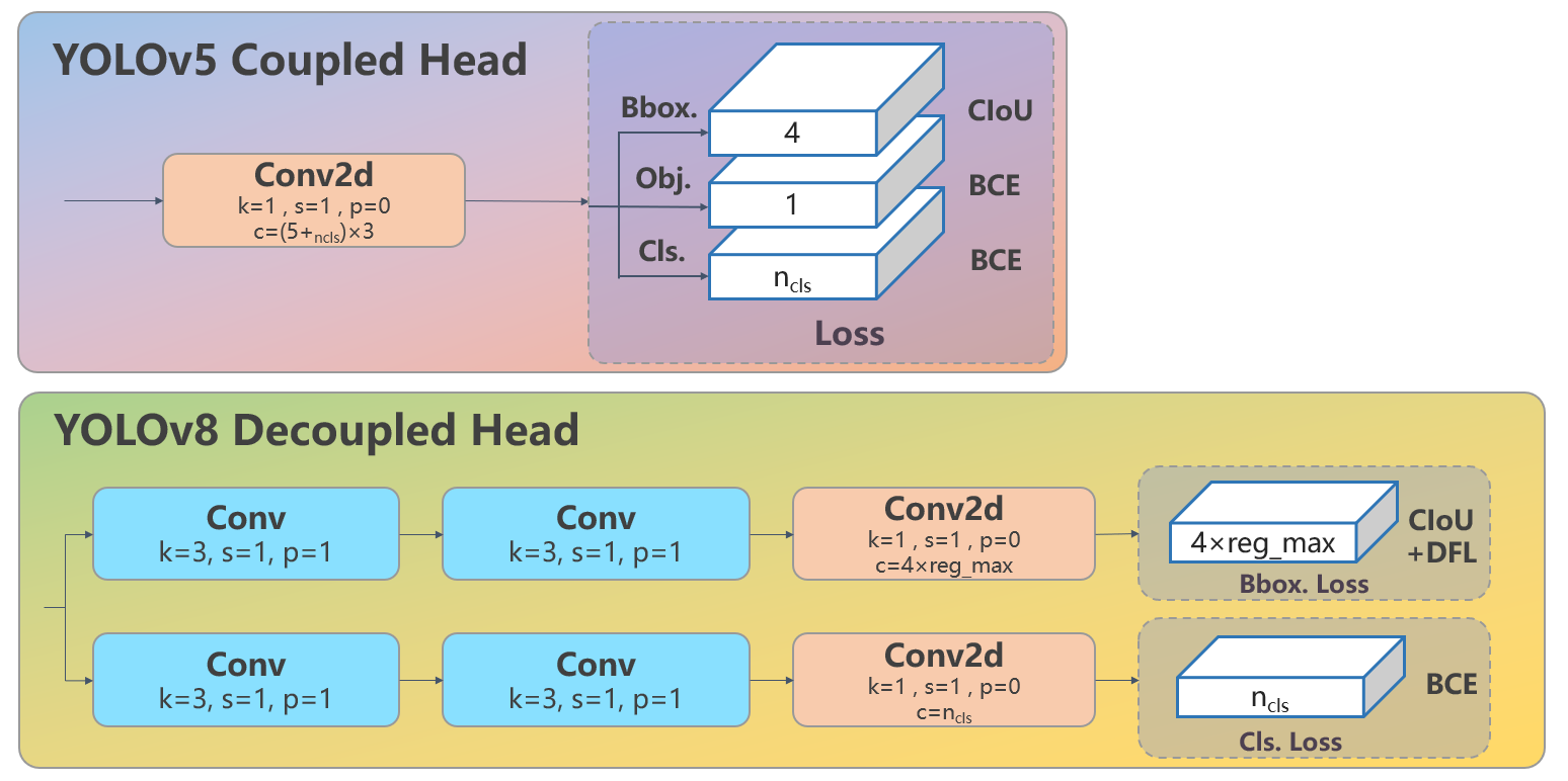
As can be seen from the figure above, in the design of the YOLOv8 decoupled detection head, the classification branch and regression branch each contain two independent 3x3 convolutional modules with a stride of 1, followed by dimensionality reduction via a 1x1 convolution according to their respective output information dimensions. For the COCO dataset, the final output data dimension of the model’s inference on a single image at the detection head is [1, 8400, 144].
Here, 1 represents the batch size; since a single image is being processed, the batch size is 1. The second value, 8400, represents the sum of all grid points across the three different scales of feature information sent from the neck network to the detection head ($80\times80 + 40\times40 + 20\times20 = 8400$). Every grid point on the feature maps outputs a 1D tensor representing the detection results at that grid point. The final 144 can be divided into two parts: the length of the category determination part is 80, corresponding to the 80 categories of the COCO dataset—the higher the class score, the more likely the detected object at that grid point belongs to that category; the length of the bounding box location detection part is 64, which is related to the Anchor-Free mechanism of the YOLOv8 detection head.
Starting from the YOLOv2 model, the first few generations of YOLO all used Anchor-based prediction box mechanisms. YOLOv8, however, adopts an Anchor-Free design and no longer relies on aspect ratios clustered from datasets to assist in locating objects. The implementation of the YOLOv8 Anchor-Free mode relies on the DFL (Distribution Focal Loss) mechanism.
The so-called DFL mechanism means that each grid output by the prediction box branch path contains the coordinate positions of the object prediction box detected by this grid. Based on the position coordinates $(x, y)$ of the current grid’s center point in the original image resolution ($640\times640$), the target coordinate positions are calculated using four offsets: $l$ (left), $t$ (top), $r$ (right), and $b$ (bottom). The top-left corner of the final predicted box coordinate position is $(x - \text{left}, y - \text{top})$, and the bottom-right corner is $(x + \text{right}, y + \text{bottom})$. Each of the four offsets $l, t, r, b$ is represented by a 16-dimensional vector, making the four offsets a 64-dimensional vector, which is the output data for each grid in the prediction box branch path.
For example, for the feature output of the P3 layer ($\text{stride} = 8$), given an anchor grid index of $(10, 20)$, the coordinates of the center point of this anchor grid in the original image are $((i + 0.5) \times \text{stride}, (j + 0.5) \times \text{stride}) = (84, 164)$. Similarly, for the P4 and P5 feature outputs, the stride must be changed to 16 and 32 respectively to calculate the coordinates of their anchor grids in the original image. These anchor coordinate positions plus the four offsets $l, t, r, b$ yield the positions of the top-left and bottom-right corners of a detection box in the original image.
So, how are the 16-dimensional vectors used to calculate these four offsets $l, t, r, b$? This involves two parameters:
reg_max: Usually set to 16, meaning the distance range of the offset from 0 to the maximum distance is evenly divided into 16 intervals.stride: The stride of the feature layer ($\text{P3}=8, \text{P4}=16, \text{P5}=32$).
Taking the P3 layer as an example to explain the offset calculation logic, its $\text{stride} = 8$, and the maximum supported offset is $16 \times 8 = 128$ pixels. These 128 pixels are divided into 16 segments at intervals of 8 pixels:
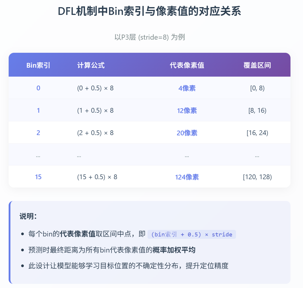
The 16-dimensional vector output by the prediction box regression branch for each offset represents the probability that the actual offset falls into each of these 16 segments. The final calculated actual offset is the weighted average of these 16 probabilities and the center points of the 16 segments (rather than simply taking the center point of the segment with the maximum probability). The logic flow for offset calculation is as follows:
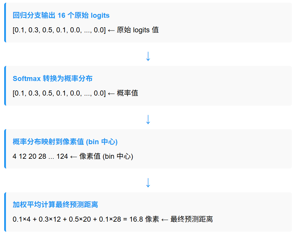
Following the above logic, the four offsets can be calculated, which, together with the center point of the anchor grid, allow us to compute the coordinates of the top-left and bottom-right corners of the predicted object bounding box detected by this anchor grid.
For the feature outputs of the P4 and P5 layers, the probability output logic and calculation logic of the offsets are completely identical, except that the strides become 16 and 32 respectively.
According to the above logic, the YOLOv8 model ultimately outputs 8400 prediction box information entries from the detection head. Such a large number of prediction boxes must subsequently pass through the NMS (Non-Maximum Suppression) algorithm filtering before serving as the final detection output of the model.
At this point, the decoupled output of the detection head is basically fully clarified: for the three multi-scale feature outputs of P3, P4, and P5, the detection head decouples them into two branches: the category determination branch and the prediction box coordinate branch. For the COCO dataset, the former outputs 80-dimensional category determination information for each grid; the latter uses a 64-dimensional vector to represent the coordinate position information of the object detected by this prediction box. Therefore, the total output dimension length for each grid is 144.
What about the object detection confidence information?
The answer is that YOLOv8 does not have an independent confidence prediction branch; instead, it hides the object detection confidence information within the class prediction information. The object detection confidence output by each grid anchor is ultimately the maximum value among the 80-dimensional tensor output by its class prediction branch—that is, the recognition probability of the class with the highest likelihood is treated as the confidence that a target exists at that anchor.