How is Millimeter Wave Radar Point Cloud Data Constructed?
- 08 Jul, 2026
The articles A Detailed Summary of Millimeter-Wave Radar FMCW Working Principles and Calculation Process and How Millimeter-Wave Radar Measures and Calculates Angle Information have comprehensively summarized the complete workflow for measuring, deriving, and calculating distance, velocity, and angular direction information using millimeter-wave radar. This article, from the perspective of using millimeter-wave radar chips and modules, summarizes how the radar’s output point cloud data is actually constructed.
Millimeter Wave Radar Output Point Cloud Data
Simply put, the point cloud data output by a millimeter-wave radar refers to a collection of data representing effective reflective targets in space, extracted from the echo radio frequency (RF) signals received by the radar’s receiving antenna after undergoing underlying digital signal processing (DSP or hardware accelerator).
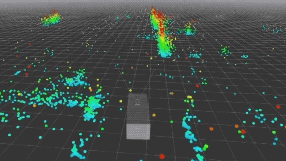
For a typical 4D millimeter-wave radar chip or module, each frame’s output point cloud consists of multiple points. The data for each point is typically a vector containing multiple dimensions of information: $P = [x, y, z, v, \text{SNR}]$.
- Spatial Coordinates ($x, y, z$): The three-dimensional spatial position of the detected target relative to the radar sensor. This is resolved by calculating the signal’s time-of-flight (range) and the phase difference between different receiving antennas (azimuth and elevation angles). How the radar measures these data points has been thoroughly summarized and explained in the articles A Detailed Summary of Millimeter-Wave Radar FMCW Working Principles and Calculation Process and How Millimeter-Wave Radar Measures and Calculates Angle Information.
- Radial Velocity ($v$): This is where millimeter-wave radar holds a competitive advantage. Relying on the Doppler effect, the radar can relatively accurately measure the instantaneous speed at which a point is approaching or receding from the sensor at a low level. It does not require estimating velocity by comparing consecutive frames, as visual algorithms do.
- Signal-to-Noise Ratio / Reflection Intensity ($\text{SNR}$ or $\text{Intensity}$, optional): Represents the strength of the signal reflected from the point. Metal objects exhibit higher reflection intensity, while objects like human bodies and fabrics show weaker reflection.
For 3D millimeter-wave radar, which only possesses a multiple-input multiple-output (MIMO) antenna array in the horizontal direction and lacks vertical antenna placement, it can only measure Range, Velocity, and Azimuth. In a Cartesian coordinate system, its output data is therefore limited to $(x, y, v)$.
Radar Chip and Module Data Output Format
Regarding the output data format for radar chips and modules, there is currently no universal data protocol or format across brands and industries. Therefore, the specific message structures output via serial port or CAN bus by different chip manufacturers (e.g., TI, NXP, Infineon) or module packagers (e.g., Sensortek, Zongmu, etc.) are proprietary.
Nevertheless, the data and information content that radar chips and modules need to output are inevitably those mentioned in the preceding sections. Consequently, the core information structure of their output data is highly consistent within the industry: most consumer-grade and automotive-grade radar modules adopt the TLV (Type-Length-Value) data structure to package point cloud frames.
The following section will illustrate the radar’s output data situation using the example of the TI mmWave sensor’s UART output data organization format, as provided in Reference [2].
Each time the radar finishes processing a frame of RF signals, it sends out a data packet. This data packet employs a classic design consisting of a fixed-length frame header plus variable-length TLV data blocks.
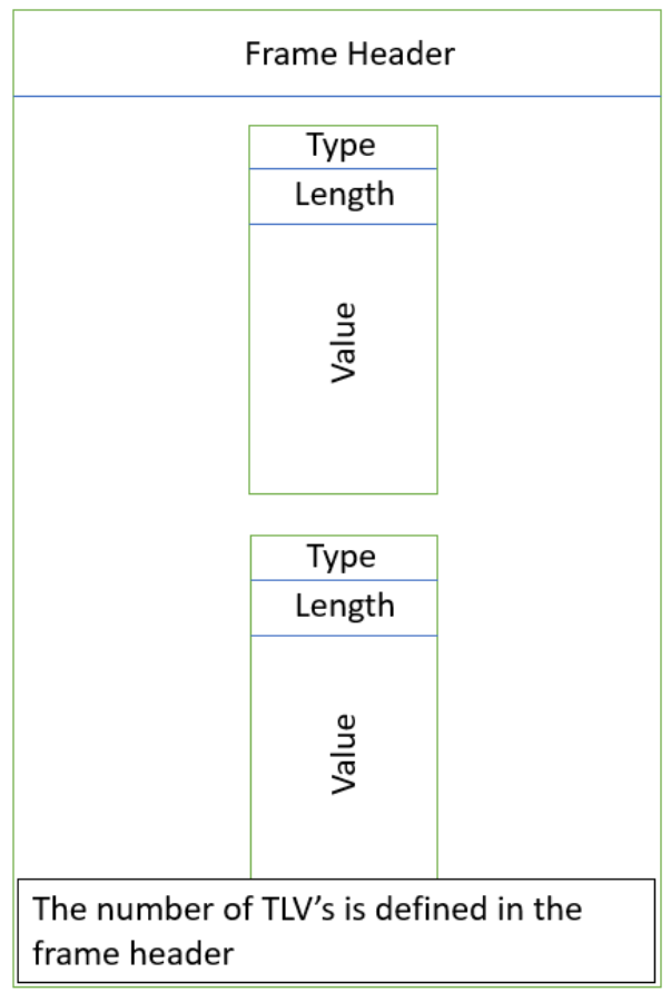
Every frame of data output begins with a fixed-length 40-byte Frame Header structure, which serves as the anchor point for parsing the radar’s data output: the total size of the data frame and the number of TLV structures contained within this frame are both defined in the Frame Header.
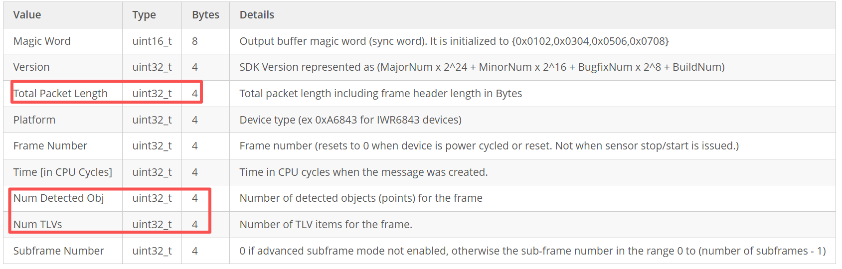
Note that Num TLVs describes how many different types of data blocks are contained in this frame data packet. Through TI’s guiMonitor command, the radar can be requested to output multiple types of data simultaneously in a single output frame, such as point cloud data (Type 1), target tracking lists (Type 1010), system status information (Type 6), etc. Each data type corresponds to one TLV structure.
Meanwhile, Num Detected Obj represents the number of valid reflective points actually detected by the radar in the physical space of the current frame. This variable is primarily used for parsing Type = 1 (Detected Points) or similar point cloud TLV data. When parsing the TLV structure containing point cloud data in a program, this variable can be used to quickly retrieve the point cloud data for all detected points.
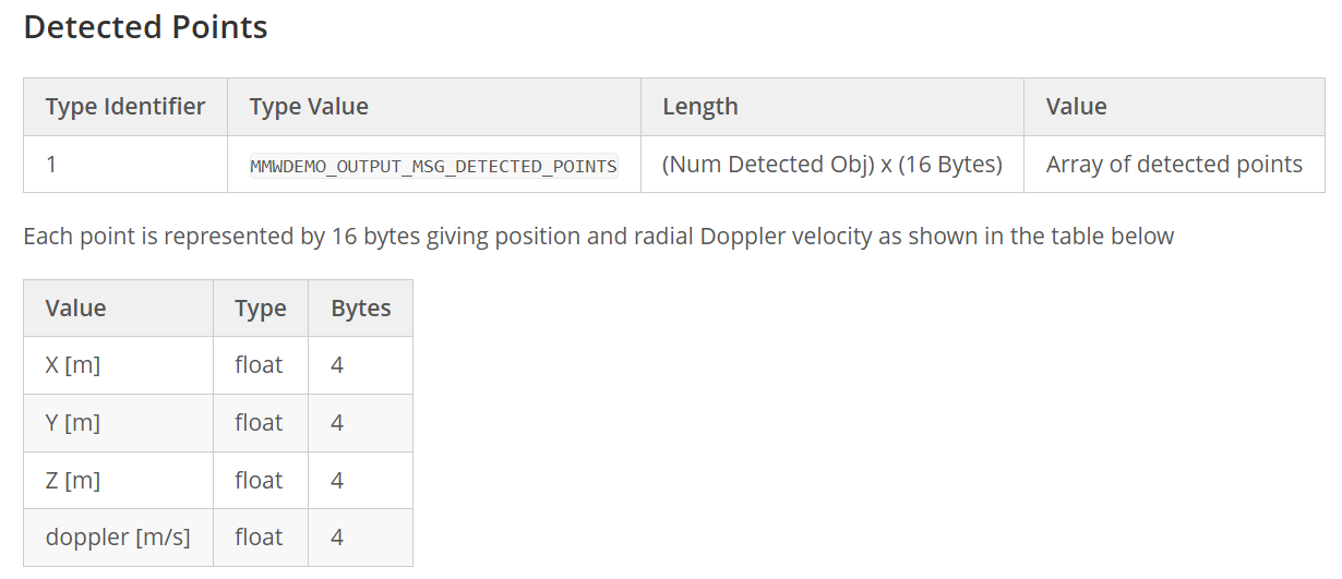
For each TLV structure, its beginning consists of a fixed 8-byte header, which contains the Type and Length information for that structure:

For the TLV structure of point cloud data, the Type field is fixed at 1, and Length represents the Data Length of this TLV structure, excluding the TLV Header.
The Data section of the TLV structure consists of contiguous point cloud data. Each point cloud data structure represents a valid detected point, with a fixed length of 16 bytes. All 4 core physical quantities for a detected point are represented using standard single-precision floating-point numbers (IEEE 754 standard). Therefore, the length of this section is 4 Bytes * Num Detected Obj.
Construction of Radar Point Cloud Information
In the real physical world, frequency-modulated continuous wave (FMCW) signals emitted by radar strike cars, pedestrians, trees, the ground, and even raindrops, and are reflected simultaneously. The radar’s receiving antenna (Rx) ultimately receives a complex analog electromagnetic wave, which is a mixture of all these reflected signals.
So, how exactly does the radar chip internally extract distinct $(x, y, z, v)$ point cloud data from this complex mixed signal?
In fact, the general calculation process has already been thoroughly summarized in the articles A Detailed Summary of Millimeter-Wave Radar FMCW Working Principles and Calculation Process and How Millimeter-Wave Radar Measures and Calculates Angle Information.
Here, we will summarize the process of constructing point cloud data from the perspective of complete point cloud information generation:
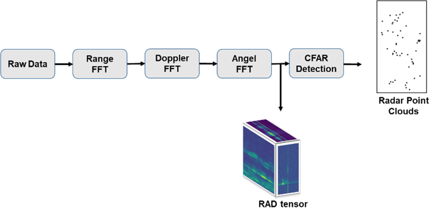
- 1D FFT (Range Dimension): After the analog signal, mixed with various echoes, is sampled by the radar’s ADC and converted into a digital signal, the first thing the DSP does is perform a Fast Fourier Transform (Range FFT). Since the frequency difference of FMCW radar echoes directly corresponds to physical distance, this step effectively slices the space by range, thus preliminarily separating objects at different distances.
- 2D FFT (Velocity Dimension): To accurately measure velocity information, the radar continuously transmits a sequence of chirps (e.g., 128 chirps forming one frame). Then, for these 128 results, another Fourier Transform (the so-called Doppler FFT) is performed in the time dimension. Because moving objects generate tiny phase differences between consecutive chirps, 2D FFT can convert these phase differences into velocity information. After the 2D FFT, the data transforms into a two-dimensional heatmap.
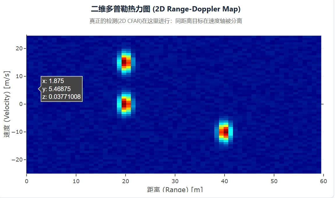
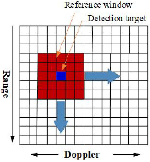
- CFAR (Constant False Alarm Rate Detection): The two-dimensional heatmap obtained from the second step, filled with varying energy levels, contains not only targets but also a significant amount of environmental background noise and ground clutter reflections. The radar must determine which are true detection targets and which are merely noise. This is where the CFAR (Constant False Alarm Rate) algorithm comes into play: when it examines a specific cell (Cell Under Test, CUT), it first evaluates the average noise level of the cells surrounding it. Only when the energy of the CUT is significantly higher than the average noise of its surrounding environment, plus a pre-set threshold, does the radar identify it as a true detection point.
- After processing with the CFAR algorithm, the radar’s detection results become discrete detection points with independent coordinates. This is the origin of millimeter-wave radar point cloud output data.
- 3D FFT (Angle Resolution): Through the calculations of the preceding three steps, the distance and velocity information of discrete detection points (point clouds) are obtained. In the final step, the radar only needs to focus on those few points that passed CFAR detection, extract the signal phase differences between different receiving antennas (Rx), and perform a third Fourier Transform to calculate the azimuth and elevation angles for that point.
Finally, each isolated detection point and energy peak possesses complete information regarding distance, velocity, angles (azimuth and elevation), and reflection intensity. This information is then packaged into standard TLV Type 1 data and transmitted via the serial port according to the protocol format described above.