How Do mmWave Radars Measure and Calculate Angle Information?

02 Jul, 2026
- Hardware

In the article Detailed Summary of FMCW mmWave Radar Sensing Workflow and Calculations, we covered the theoretical derivations and mathematical formulas for detecting target range and velocity using millimeter-wave (mmWave) radar. This article provides a comprehensive breakdown of the angle concepts within mmWave radar point cloud data, as well as the complete calculation workflow for angle estimation.

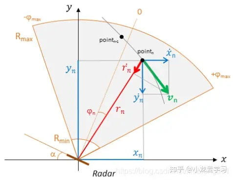
Definition of Angle

In the point cloud data output by mmWave radar, the embedded angle information essentially refers to the Angle of Arrival (AoA) of the electromagnetic waves reflected back from the target.

In 3D spatial applications, this angle information typically covers two dimensions:

Azimuth (Horizontal Angle): The angular displacement of the target relative to the radar’s horizontal plane (left/right). For example, the radar detects a vehicle 15° to the left of dead center.
Elevation (Vertical Angle): The angular displacement of the target relative to the radar’s vertical plane (up/down). For example, the radar detects an overpass or road sign 10° above dead center.

With the three spherical coordinates—range R, azimuth φ, and elevation θ—combined with the radar’s own position, we can convert these values into Cartesian coordinates (x, y, z). This coordinate transformation is precisely why the radar’s point cloud output can render spatial contours of targets in 3D space.

Working Principle of Radar Angle Estimation

A single radar antenna relies on the frequency difference of Frequency-Modulated Continuous Waves (FMCW) to measure range, and Doppler frequency shifts (phase differences) to measure velocity. However, a single antenna alone cannot estimate angles.

To obtain angle information, a radar must rely on multi-antenna arrays (MIMO technology, i.e., multiple transmit antennas TX and multiple receive antennas RX). The core angle estimation technique is based on phase-difference-based Angle of Arrival (AoA) measurement.

When the electromagnetic waves emitted by the radar’s transmit antenna hit a target and bounce back, the reflected signal reaches the radar’s multiple receive antennas as a set of roughly parallel electromagnetic waves (plane waves).

Suppose a target object is located at an angle $\theta$ relative to the radar’s boresight. Because the receive antennas on the radar board are spaced at a fixed physical distance $d$ (typically designed as half a wavelength $\frac{\lambda}{2}$), there will be a tiny time difference between when the echo reaches adjacent antennas: after reaching the first receive antenna (RX1), the wave must travel a tiny additional distance before reaching the second receive antenna (RX2).

Assuming the physical distance between two receive antennas is $L$, trigonometric functions on a right triangle tell us that this additional path length (path length difference) is $\Delta d = L \cdot \sin(\theta)$.

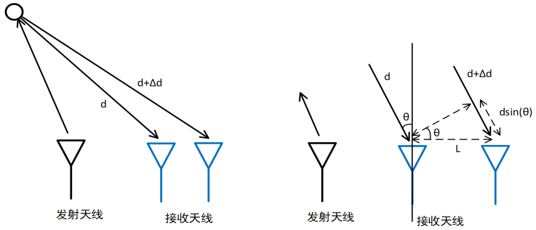
Because electromagnetic waves are sinusoidal, traveling this extra distance $\Delta d$ manifests as a phase shift in the received signal (meaning there is a constant phase difference between the signals received by the two antennas). A full wavelength $\lambda$ corresponds to a complete cycle ($2\pi$ phase). Thus, traveling an extra distance $\Delta d$ corresponds to a phase difference $\Delta \phi$ of:

$$ \Delta \phi = \frac{2\pi}{\lambda} \cdot \Delta x = \frac{2\pi \cdot L \cdot \sin(\theta)}{\lambda} $$

Next, we solve for the angle $\theta$ from the equation above. Since the radar hardware chip can accurately measure the phase difference $\Delta \phi$ between the signals received by RX1 and RX2 (by sampling and running an FFT on the waveforms received by RX1 and RX2—similar to range calculation—extracting the phase from the FFT results, and then calculating the phase difference), the inter-antenna spacing $L$ is fixed by design, and the wavelength $\lambda$ of the emitted electromagnetic wave is also constant, we can easily calculate the target angle $\theta$ using the formula below:

$$ \theta = \arcsin\left(\frac{\Delta \phi \cdot \lambda}{2\pi \cdot L}\right) $$

This is the underlying essence of radar angle estimation: measuring the phase difference between signals received by different antennas and using trigonometric functions to calculate the target’s angle.

3D Radar vs. 4D Radar

The angle measurement principle outlined above is quite straightforward, but there is an important caveat: if the radar’s receive antennas are arranged in a single horizontal row, it can only measure the azimuth (horizontal angle). This is what is known as a 3D radar.

The reason is simple: when all receive antennas are aligned along the same horizontal line, there is only horizontal spacing between them. Under these conditions:

When a target moves left or right (azimuth), the path lengths traveled by the electromagnetic wave to each antenna vary, creating phase differences. The radar can then compute the azimuth angle following the workflow described above.
However, when a target moves up or down (elevation), because the reflected electromagnetic plane wave arrives in parallel from above or below, the distance it travels to each horizontally aligned antenna is identical. Consequently, the phase difference generated in the vertical direction is zero. The radar cannot distinguish whether the target is overhead or on the ground. This explains why traditional 3D radars in automotive applications often confuse overhead bridges with road-level obstacles.

4D radar introduces vertical sensing capability on top of 3D radar capabilities. In practical system design, clever 2D Planar Arrays or MIMO (Multiple-Input Multiple-Output) virtual antenna techniques are typically employed. In terms of antenna array design, the transmit (TX) and receive (RX) antennas are arranged in a staggered pattern, with intentional height differences designed into the transmit antennas. When multiple transmit and receive antennas operate simultaneously, algorithms combine them to synthesize a larger number of virtual antenna points, forming a two-dimensional planar array in both horizontal and vertical directions.

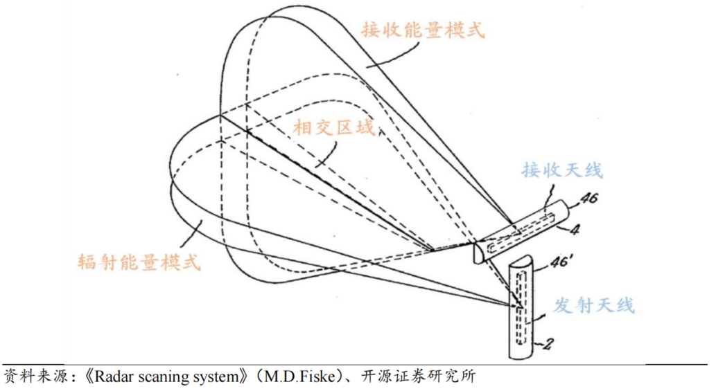
The horizontally extended virtual antenna array leverages horizontal distance differences to measure the horizontal azimuth, while the vertically extended virtual array (with height offsets) leverages vertical distance differences to measure the vertical elevation.

To summarize, the radar industry defines radar dimensions (D) as follows:

3D Radar measures 3 dimensions: Range, Velocity (Doppler), and Azimuth.
4D Radar measures 4 dimensions: Range, Velocity, Azimuth, and Elevation.

The 3D spatial coordinates (X, Y, Z) commonly seen in radar point cloud data are calculated precisely from these three physical quantities—range, azimuth, and elevation—using trigonometric transformations.

Radar Angular Resolution

Just like range and velocity measurements, radar angle measurement also has a concept of minimum resolution: angular resolution.

In radar engineering, Angular Resolution refers to the minimum angular separation required between two adjacent targets at the same range and velocity for the radar to distinguish them as separate entities. If two targets (such as a pedestrian and a parked car next to them) have an angular separation smaller than the radar’s angular resolution, the radar’s DSP will treat them as a single echo peak, outputting a single merged point in the point cloud data rather than two distinct targets.

Modern 4D imaging radars mostly adopt single-chip large array designs (such as 4TX/4RX or 4TX/6RX) or even multi-chip cascaded antenna designs (e.g., combining 4 chips to achieve 12TX/16RX). Their horizontal azimuth resolution can reach high precisions of 1° to 1.5°, while vertical elevation resolution typically falls between 2° and 5°.

How to Calculate Angular Resolution?

In radar and antenna theory, angular resolution is fundamentally determined by the mainlobe width of the antenna array. Rayleigh’s criterion in physics states that two targets are resolvable when the peak of one target’s beam pattern coincides with the first null (zero point) of the other.

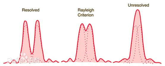
For a uniform linear array (ULA) of length $D$, its antenna pattern (beam shape) can be described using a $\text{sinc}$ function. The theoretical formula for its 3dB beamwidth (the angular width where power drops by half, defined as the angular resolution $\theta_{res}$ in engineering) is:

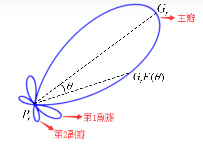
$$ \theta_{res} \text{ (radians)} \approx 0.886 \frac{\lambda}{D} $$

For quick engineering estimations, the factor $0.886$ is often omitted, yielding the approximation:

$$ \theta_{res} \approx \frac{\lambda}{D} $$

Since $\pi \text{ radians} = 180^\circ$, 1 radian $= \frac{180^\circ}{\pi} \approx 57.3^\circ$. Substituting this into the equation above gives the formula in degrees:

$$ \theta_{res} \text{ (degrees)} \approx 57.3^\circ \times \frac{\lambda}{D} $$

Assuming there are $N$ receive antennas spaced at $d = \frac{\lambda}{2}$, the effective aperture length of the array is:

$$ D = N \cdot d = N \cdot \frac{\lambda}{2} $$

Substituting $D$ back into the degree-based resolution formula yields:

$$ \theta_{res} \text{ (degrees)} \approx 57.3^\circ \times \frac{\lambda}{N \cdot \frac{\lambda}{2}} = \frac{114.6^\circ}{N} $$

This serves as a rule-of-thumb formula for quickly calculating radar angular resolution in engineering practice. As shown, the only way to improve angular resolution is to increase the number of receive antennas $N$.

According to this quick formula, achieving a 1° angular resolution would require 114 receive antennas spaced at $\frac{\lambda}{2}$—which is practically impossible on a compact circuit board. This brings us to MIMO (Multiple-Input Multiple-Output) and Virtual Antenna Array technology.

MIMO Virtual Antenna Arrays

In radar antenna design, packing a massive number of physical receive antennas into hardware is impractical. However, in engineering practice, a small number of transmit (TX) and receive (RX) antennas can be multiplied together to synthesize a large virtual antenna array within the radar processing pipeline, thereby dramatically boosting angular resolution.

The general workflow is as follows:

Transmit antenna TX1 sends a chirp signal, and the 4 physical receive antennas (RX1–RX4) on the board capture the reflection. At this moment, the system acquires 4 spatial phase samples.
A fraction of a second later, TX1 stops and TX2 transmits a signal. During PCB layout design, TX2’s physical position is intentionally shifted laterally by a precise distance (typically 4 times half a wavelength). Thus, when TX2 transmits a signal that hits the target and reflects back to RX1–RX4, the electromagnetic wave travels an extra distance due to TX2’s spatial offset.
When the radar’s DSP processes the signal, the phases received by RX1–RX4 during TX2’s transmission are mathematically equivalent to phases that would be received by 4 new virtual receive antennas (RX5–RX8) placed directly to the right of TX1.

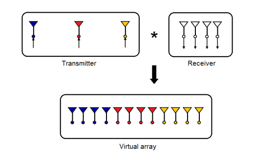
Therefore, by having 3 TX antennas transmit sequentially in time combined with 4 RX antennas receiving, the radar software successfully reconstructs phase data for $3 \times 4 = 12$ virtual antennas.

Using flagship single-chip solutions from vendors like TI or NXP (e.g., 4TX / 4RX), MIMO techniques can synthesize up to 16 virtual antennas ($114^\circ / 16 \approx 7.1^\circ$ resolution).

Furthermore, if 4 such chips are cascaded (e.g., achieving 12TX and 16RX), they can synthesize $12 \times 16 = 192$ virtual antennas.

This virtual antenna approach is precisely how modern flagship 4D imaging radars achieve high-precision horizontal and vertical angular resolutions.