Detailed Summary of FMCW mmWave Radar Principles and Calculation Process

In the article Understanding the Principles and Applications of mmWave Sensing Radar, we briefly summarized the fundamental principles of radar and millimeter-wave (mmWave) radar, as well as the calculation processes for its two operating modes. This article provides a detailed summary of the working principles, range, and velocity calculation workflows of the FMCW mode in mmWave sensing. This will help build a deeper understanding of the concepts and operating procedures of this radar mode.

Structure and Organization of FMCW Transmit Signals

As summarized in Understanding the Principles and Applications of mmWave Sensing Radar, in the FMCW (Frequency Modulated Continuous Wave) mode of mmWave radar, the radar does not transmit traditional discrete pulses. Instead, it transmits a continuous sine wave whose frequency increases linearly over time, known as a Chirp signal.

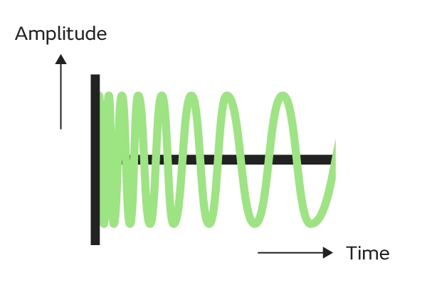
The core physical characteristics of a chirp can be defined by the following parameters:

• Start Frequency ($f_c$): e.g., 77 GHz.
• Bandwidth ($B$): The frequency sweep range, e.g., 4 GHz. Bandwidth determines the radar’s Range Resolution. A higher bandwidth yields a finer range resolution, making it easier to distinguish two closely spaced objects.
• Ramp Time / Duration ($T_c$): The time taken for the frequency to sweep from $f_c$ to $f_c + B$, e.g., 40 µs.
• Frequency Slope ($S$): The rate of frequency change, calculated as $S = \frac{B}{T_c}$.

A single chirp is sufficient if you only need to measure the distance to a static object. However, to measure the velocity of a moving object, multiple consecutive chirps are required. Therefore, radar data is organized into frames (Frames). Each Frame contains multiple consecutive chirp signals, facilitating periodic data throughput and object detection for subsequent processing by an NPU or DSP.

For a single chirp signal, its microscopic timeline mainly consists of the following two phases:

• Inter Chirp Idle Time: The transmitter does not transmit active signals, and the frequency synthesizer quickly ramps back down and locks onto the start frequency $f_c$.
• Tx Start: The transmitter turns on, and the frequency begins to rise linearly from $f_c$ to $f_c + B$.

A Frame consists of a sequence of identical, consecutive chirp signals. The key parameters of a Frame are as follows:

• Number of Chirps (per frame): e.g., 128 chirps per frame. This value determines the radar’s velocity resolution.
• Frame Periodicity: e.g., 33 ms (corresponding to approximately 30 FPS).
• Active Frame Time: The duration occupied by transmitting 128 chirps consecutively.
• Inter-Frame Time: The gap between the end of one frame and the start of the next. During this time, the radar’s RF front-end typically enters a low-power state, while the backend processor (such as a DSP, ARM, or NPU) works at full speed to process the raw ADC data generated during the active frame.

The figure below shows the timeline structure of a Frame containing consecutive chirp signals:

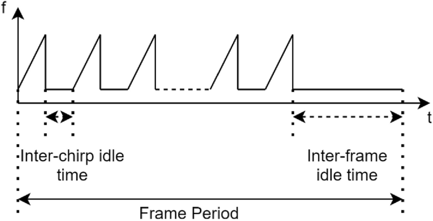
Below is an example illustrating the timeline of chirps and frames transmitted by the radar:

• Chirp Duration ($T_c$): 50 µs
• Chirp Idle Time: 10 µs (Thus, the total period to transmit a single complete chirp is 60 µs)
• Number of Chirps per Frame: 128
• Active Transmission Time: $60 , \mu s \times 128 = 7.68$ ms
• Frame Periodicity: 33 ms

Based on these parameters, the transmitter operation workflow of the radar system is as follows: within every 33 ms period, the transmitter only operates during the first 7.68 ms, transmitting 128 chirps continuously at rapid intervals (60 µs). During the remaining ~25 ms, the transmitter is turned off, waiting for the next frame trigger.

Radar System Architecture and Intermediate Frequency (IF) Signal

The architecture of an FMCW mmWave radar system is shown in the diagram below:

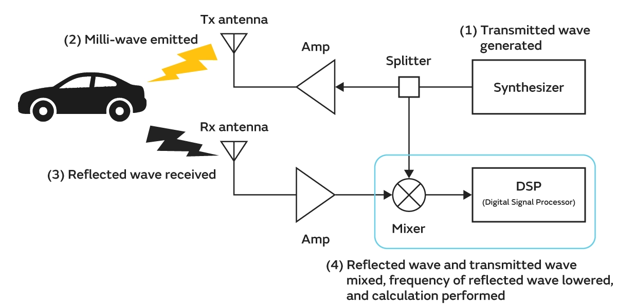
The Mixer in this block diagram multiplies (mixes) the current transmitted signal with the received echo signal. The mixed signal then passes through a low-pass filter to generate an Intermediate Frequency (IF) signal, which is used for subsequent calculations.

Suppose the transmitted signal at the current moment is $S_{TX} = \cos(2\pi f_{TX} t+\phi_{TX})$, and the received echo signal is $S_{RX} = \cos(2\pi f_{RX} t+\phi_{RX})$.

The intermediate frequency (IF) signal obtained after mixing and low-pass filtering is:

$$ S_{out} = \cos(2\pi (f_{TX} - f_{RX}) t+(\phi_{TX}-\phi_{RX})) $$

Subsequent calculations for range, velocity, and angle are all performed based on this IF signal.

Range Calculation Workflow

The key to understanding range calculation is that the received RX signal is a time-delayed version of the transmitted TX signal.

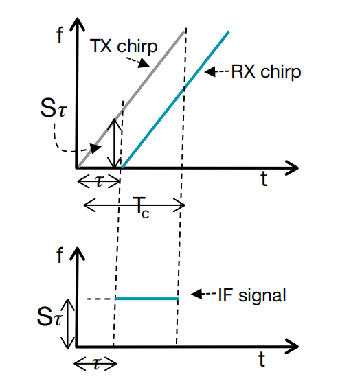
Assuming the round-trip time-of-flight of the electromagnetic wave from the transmitter to the target and back to the receiver is $\tau$, the time delay formula is $\tau = \frac{2d}{c}$, where $d$ is the distance to the object and $c$ is the speed of light.

Since the frequency of the TX signal increases linearly with time, subtracting the RX signal (which is delayed by $\tau$) from the TX signal at any given instant yields a constant frequency difference. This frequency difference is the frequency of the IF signal.

Based on geometric similarity, the frequency of the IF signal $f_0$ is equal to the slope $S$ multiplied by the time delay $\tau$. Combining this with the time delay formula above yields the final range calculation formula:

$$ f_0 = \frac{S \cdot 2d}{c} $$

Thus, by extracting the frequency $f_0$ of the IF signal, the system can directly compute the range $d$ to the target.

DSP Computation Workflow

The DSP computation workflow for range is as follows:

• ADC Sampling: The analog mixer outputs an analog intermediate frequency (IF) sine wave, which the DSP must first digitize using an ADC (Analog-to-Digital Converter). Given an ADC sampling rate $F_s$ (e.g., 6.4 Msps) and the number of sample points per chirp $N$ (e.g., 256 points), this step yields an array of length $N$.
• Signal Windowing: Before performing the FFT, to mitigate spectral leakage caused by computing FFTs on finite-length arrays, the $N$ sample points are typically multiplied by a window function of the same length (such as a Hanning or Blackman window).
• FFT Execution: The DSP’s hardware accelerator (HWA) or DSP core performs a Discrete Fourier Transform (DFT/FFT) on the $N$ windowed time-domain data points. This produces a frequency-domain array of $N$ complex numbers (real + imaginary parts). According to the Nyquist theorem, we typically only need to inspect the first $N/2$ points. In radar terminology, these $N/2$ points are referred to as Range Bins or Index $k$.
• Magnitude Calculation & Peak Detection: The FFT output is in the complex domain, representing both phase and magnitude. The DSP traverses these $N/2$ Range Bins and calculates the magnitude of each point as $A = \sqrt{I^2 + Q^2}$. In the simplified scenario of a single detected target, the DSP only needs to identify the bin with the largest value (highest energy) among the $N/2$ points and record its index, denoted as Index $k$.
  • If multiple targets are present, scanning the FFT magnitudes will reveal multiple peaks. In this case, the DSP records the indices of all these peak points.
• Physical Metric Conversion: This step converts the index obtained in the previous step into a physical distance in meters (m), using the following conversion workflow.

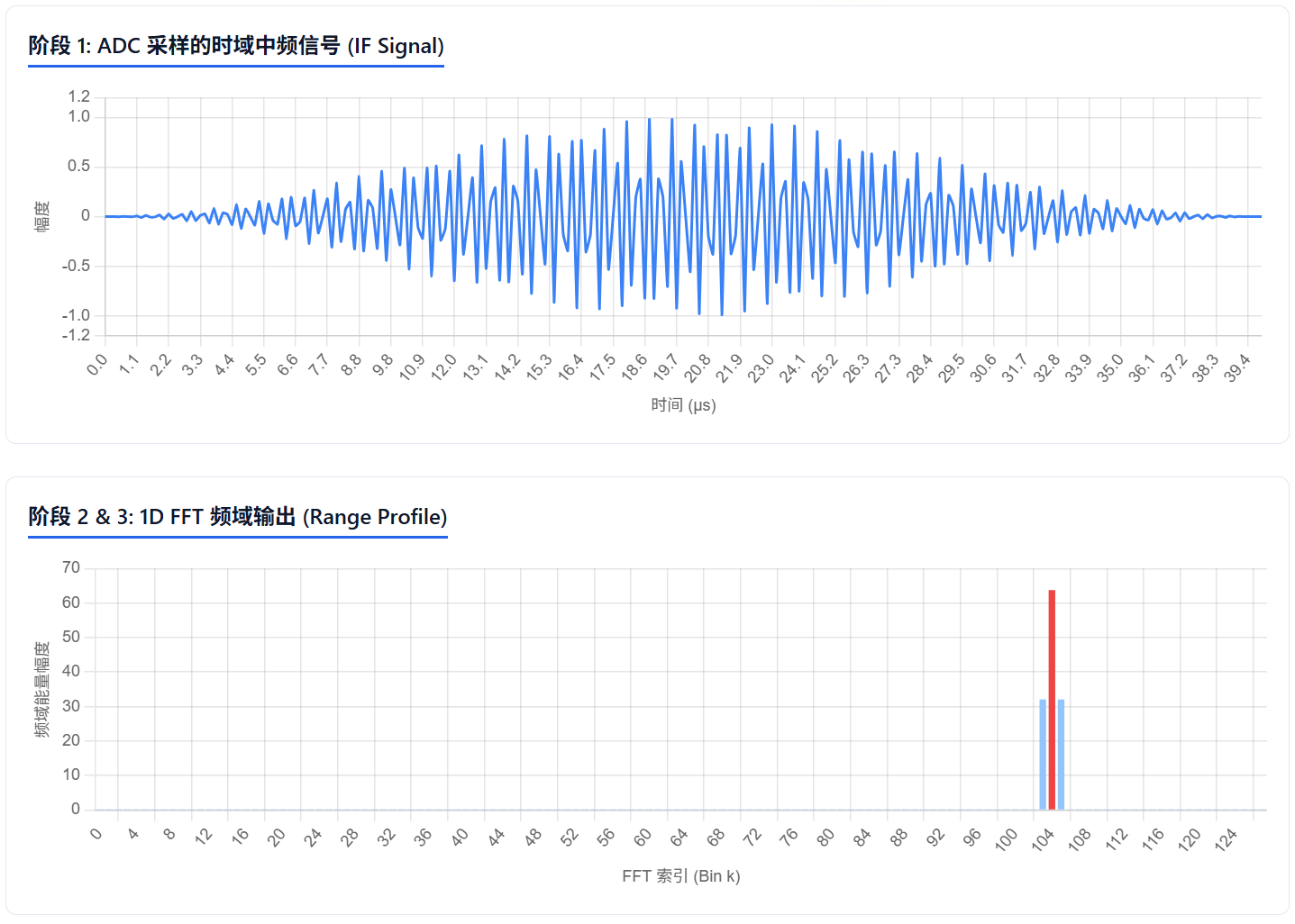
The frequency span represented by each bin (frequency resolution $\Delta f$) is determined by the ADC parameters: $\Delta f = \frac{F_s}{N}$, where $F_s$ is the ADC sampling rate.

Therefore, the IF frequency corresponding to the peak (located at Range Bin index $k$) is: $f_{IF} = k \times \Delta f = k \times \frac{F_s}{N}$.

Combining this with the radar range formula ($f_{IF} = \frac{S \cdot 2d}{c}$) and rearranging for distance $d$ yields: $d = \frac{c \cdot f_{IF}}{2S}$.

The final range calculation formula is:

$$ Distance = k \times \left( \frac{c \cdot F_s}{2 \cdot S \cdot N} \right) $$

The term in parentheses $\frac{c \cdot F_s}{2 \cdot S \cdot N}$** is a constant determined during radar initialization. This constant represents the radar’s range resolution per single bin ($\Delta d$).**

Velocity Calculation Workflow

Since the range of an object can be determined from a single chirp measurement, can we easily calculate the velocity of a moving object by comparing the range across multiple chirps? The answer is no.

Suppose a target is moving at velocity $v$, and the radar transmits two identical, consecutive chirps separated by an interval of $T_c$ (the chirp period). Within the extremely short interval between the first and second chirp (e.g., 60 µs), the target moves only an infinitesimally small distance: $\Delta d = v \cdot T_c$. For typical moving objects, this distance is on the scale of micrometers. Such a tiny difference in distance is invisible as a frequency shift on the 1D FFT spectrum; hence, the peaks of both chirps will still appear in the exact same Range Bin.

However, because the wavelength of the millimeter wave $\lambda$ is extremely short (approximately 3.9 mm at 77 GHz), this minute difference in distance produces a prominent phase shift $\Delta \phi$ between the IF signals of the two chirps in the complex domain.

As an electromagnetic wave travels a physical distance $d$ in space, its phase changes by:

$$ 2\pi \times \frac{d}{\lambda} $$

Suppose the physical distance between the radar and the target is $d$. However, the transmitted chirp signal must travel to the target and then reflect back to the receiving antenna. Thus, the actual total round-trip path of the electromagnetic wave through the air is $2d$.

Substituting the total path distance $2d$ into the initial equation, and considering the tiny distance moved by the target $\Delta d = v \times T_c$, we derive the physical formula for the phase difference in the received signals:

$$ \Delta \phi = \frac{4\pi \Delta d}{\lambda} = \frac{4\pi v T_c}{\lambda} $$

From this formula, we can back-calculate the target velocity $v$:

$$ v = \frac{\lambda \Delta\Phi}{4\pi T_c} $$

Based on the formula above, the velocity of the target can be calculated as long as we extract the phase difference between the two chirp signals.

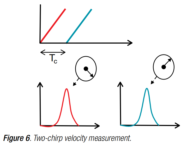
💡 Here, the concept of Maximum Unambiguous Velocity ($v_{max}$) comes into play. Since phase is calculated via trigonometric functions, it is periodic. To guarantee uniqueness in velocity measurement (preventing velocity ambiguity), the absolute phase difference between two consecutive samples must be less than $\pi$. From this, we can derive the maximum relative velocity the radar can measure: $v_{max} = \frac{\lambda}{4T_c}$. This implies that a shorter chirp period $T_c$ (more densely spaced transmissions) enables the measurement of higher maximum velocities.

DSP Computation Workflow

The DSP computation workflow for velocity is as follows:

• Constructing the Radar Data Matrix: Within a single frame, the ADC collects $M$ chirps (e.g., 128), with each chirp containing $N$ sample points (e.g., 256). The DSP first performs a 1D FFT (Range FFT) on the 256 time-domain sample points of each chirp. The complex FFT outputs (containing magnitude and phase) for each chirp are written to memory and assembled into a 2D matrix of size $M \times (N/2)$.
• Range Bin Locking & Data Extraction: Within the brief duration of a single frame (which is typically only a few milliseconds), the physical displacement of a normally moving target is extremely small, meaning it generally will not cross the radar’s range resolution cells. Assuming that the target’s energy peak is found at the $k$-th Range Bin across the FFT output sequences of all chirps, this step extracts the complex data (containing both magnitude and phase) at this $k$-th bin across all $M$ chirps, forming a new 1D complex array of length $M$.
• Windowing: Similar to the range calculation logic, to prevent spectral leakage during the subsequent 2D FFT calculation, the DSP multiplies each element of this 1D complex array of length $M$ by the coefficients of a 1-dimensional window function (e.g., a Hanning window).
• 2D FFT (Doppler FFT) Execution: The DSP’s Fourier transform unit performs an $M$-point FFT (commonly referred to as a 2D FFT) on this windowed complex array of length $M$. The result is a complex array of length $M$, where each element represents a specific Doppler Bin.
• Peak Detection & Velocity Metric Conversion: The DSP calculates the magnitude of each element in the 2D FFT output array ($A = \sqrt{I^2 + Q^2}$) to construct a velocity power spectrum. It then identifies the index of the Doppler Bin with the highest energy, denoted as Index $m$.

The velocity power spectrum calculated through the 2D FFT contains $M$ bins, which physically corresponds to dividing the full $2\pi$ phase cycle into $M$ discrete parts. Based on the phase difference formula above, the equation for each phase step is:

$$ \Delta \phi = \frac{4\pi v T_c}{\lambda} = \frac{2\pi}{M} $$

Thus, the resulting velocity resolution (which represents the physical velocity step per bin in the velocity power spectrum) is:

$$ \Delta v = \frac{\lambda}{2 \cdot M \cdot T_c} $$

Given that the peak in the velocity power spectrum lies at the $m$-th bin, the corresponding target velocity is calculated as:

$$ Velocity = m \times \Delta v = m \times \left( \frac{\lambda}{2 \cdot M \cdot T_c} \right) $$

What If There Are Multiple Targets?

The summary of range and velocity calculations above assumed a simplified scenario containing only a single target. What happens if there are multiple targets in the scene simultaneously?

In this scenario, measuring the distances to the targets is relatively straightforward.

If multiple targets are present, after receiving the reflected echoes, sampling via the ADC, and performing the 1D FFT on the DSP, multiple distinct peaks at different indices will emerge on the range spectrum (Range Bins). Each peak corresponds to the distance of a specific detected target.

However, if two objects are located too close together—closer than the radar’s range resolution limit—they will merge into the same Range Bin index. In this case, the radar cannot resolve them separately, and they will be represented as a single target.

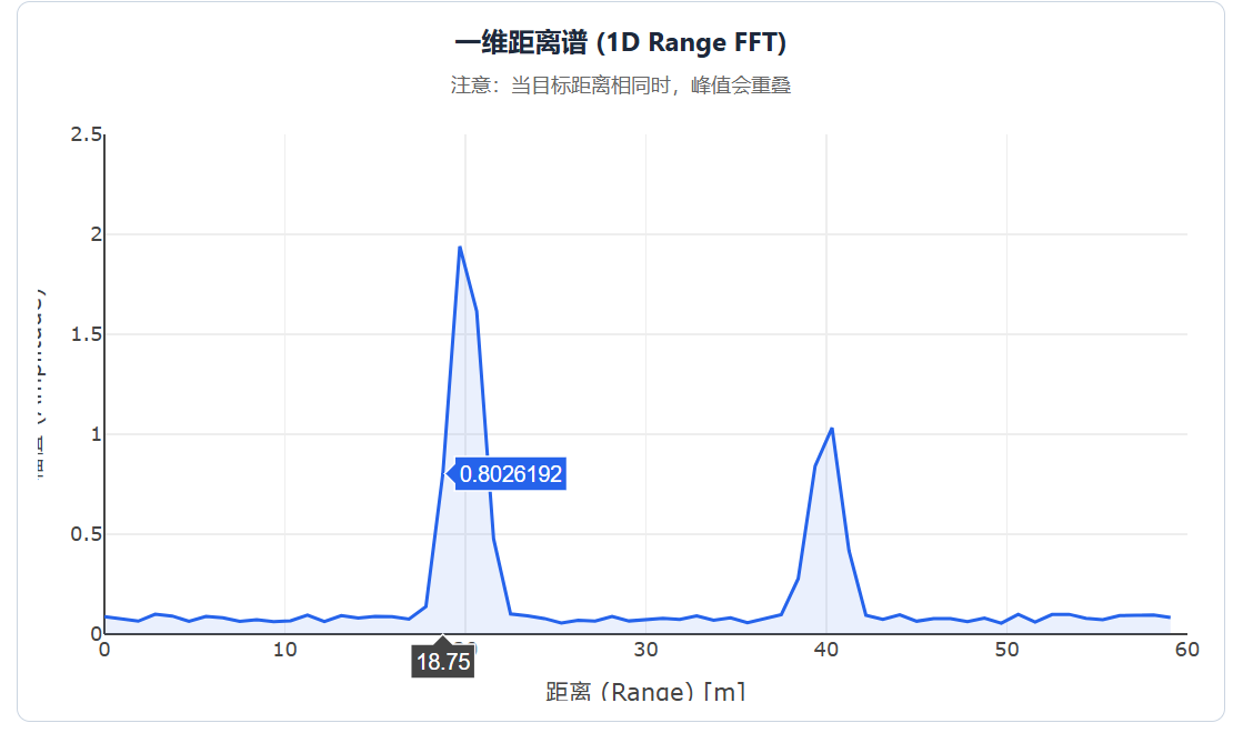
But what if two targets are at the exact same distance but moving at different velocities? Since their signals share a single Range Bin, the extracted phase sequence will be a convoluted overlay of both target phases, preventing the radar from correctly resolving and identifying their individual velocities.

To measure velocity under these conditions, instead of first finding peak bins in the range spectrum and only calculating the 2D FFT for those specific bins across all chirps, the system must perform the following:

• Perform a 1D FFT (Range FFT) on all $M$ chirps within the entire frame and stack the results to construct a 2D Radar Data Matrix (where rows represent Range Bins and columns represent Chirps).
  • Each column of this 2D matrix corresponds to a single chirp. Looking across columns for a specific Range Bin reveals how the magnitude and phase of the detected target evolve over $M$ consecutive chirps within a frame. Because the frame duration is very short, the magnitude changes in this sequence are negligible, but the phase exhibits significant variation depending on the target’s velocity.
  • If a single Range Bin contains multiple targets, the phase and amplitude in this sequence represent the superimposed vector sum of those targets.
• Execute a 2D FFT (Doppler FFT) across every row (each Range Bin) of the Data Matrix.
  • If a Range Bin contains only one target, the 2D FFT maps its phase variation to its corresponding velocity.
  • If a Range Bin contains multiple targets, the 2D FFT can successfully decompose and separate the phase shifts caused by their distinct velocities.
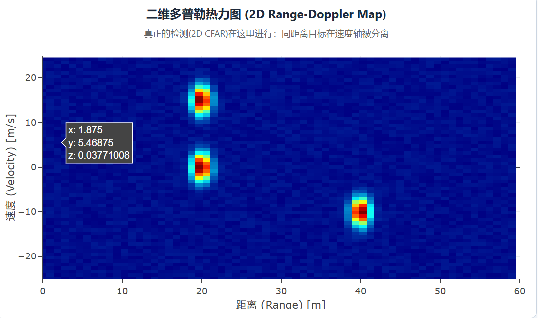
• After performing the 2D FFT on the entire matrix, the DSP generates a 2D Range-Doppler heat map in memory, where the horizontal axis represents range, the vertical axis represents velocity, and the color intensity denotes energy (amplitude).
• Finally, the system performs peak detection directly on this 2D heat map. Each 2D peak corresponds to the range and velocity data of an individual detected target.

As shown, on this heat map, two objects situated at the exact same Range Bin but moving at different velocities can be clearly resolved and identified.

References

• The fundamentals of millimeter wave radar sensors, Texas Instruments.