Summary of Preliminary Research on the PANNs Audio Classification Model
- 26 Mar, 2026
This article organizes the basic information of the classic audio classification model PANNs, its model architecture, the classification of pre-trained parameter files, the setup of the development environment, basic inference testing, and explains the network architecture of its flagship CNN14 model.
Introduction to the PANNs Model
PANNs stands for Large-scale Pre-trained Audio Neural Networks. Proposed by Qiuqiang Kong and other researchers between 2019 and 2020, its core significance lies in breaking the deadlock of “small samples and difficult training” in the audio field, providing a powerful general-purpose feature extractor for various audio tasks. In terms of the overall workflow, its working principle is equivalent to first generating a corresponding Mel-scale spectrogram for the audio file, and then using a standard convolutional neural network to perform classification tasks based on this spectrogram. The GitHub repository for this model is: qiuqiangkong/audioset_tagging_cnn
The PANNs model is powerful because it has been extensively trained on Google’s AudioSet dataset, learning to distinguish the spectral features of almost all common sounds in the world. The download link for the model’s pre-trained parameter files is: PANNs: Large-Scale Pretrained Audio Neural Networks for Audio Pattern Recognition (Pretrained Models). As can be seen from the pre-trained parameter download file list above, the model provides pre-trained parameter files for multiple different network models and parameters:
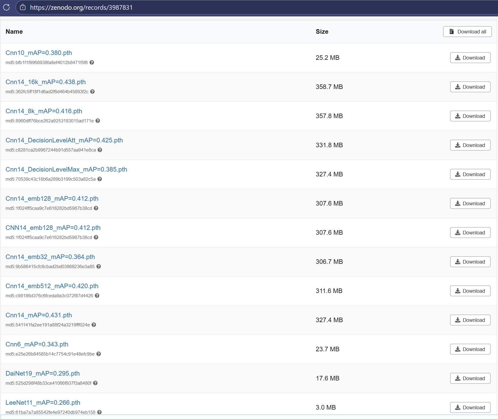
The naming format of these pre-trained parameter files is generally: ModelArchitecture_SampleRate_EmbeddingSize_PerformanceMetric.pth.
- Model Architecture: Supported model architecture versions include CNN14 (recommended model architecture), CNN6/CNN10 (lightweight versions), ResNet/MobileNet, Wavegram-Logmel-Cnn14 (high performance, but computationally intensive), and DecisionLevelMax (suitable for Sound Event Detection inference mode).
- Sample Rate: PANNs’ official implementation presets support for three sample rates: 8kHz, 16kHz, and 32kHz, with 32kHz as the default sample rate.
- Embedding Vector Length: The dimension of the embedding vector entering the detection head, with 2048 as the default. The official weight file repository also provides support for dimensions of 32, 128, and 512.
- Performance Metric: The mAP metric tested on Google’s AudioSet data validation set.
Environment Installation and Basic Inference Testing
Environment and dependency installation:
https://github.com/qiuqiangkong/audioset_tagging_cnn.git
pip install -r requirements.txt
pip install h5py  # This package needs to be installed additionally, otherwise subsequent demo runs will throw errors
As seen from the scripts/0_inference.sh script in the source code directory, the inference mode of this model can be divided into two modes: Audio Tagging and Sound Event Detection.
- Audio Tagging:
- The problem it solves is: What is the content of this recording.
- The model output result is the overall classification probability of the entire audio segment, corresponding to the 527 audio categories in Google’s AudioSet dataset.
- Its technical judgment logic performs global pooling on the audio file across the entire time dimension, providing only a single overall classification probability judgment.
- Sound Event Detection (SED):
- The problem it solves is: When did a specific audio event occur.
- The model output result is a timeline, marking the start and end times of abnormal sound occurrences on this timeline.
- Its technical implementation logic builds upon Audio Tagging by preserving time resolution and then judging audio events across the entire time period frame by frame like a scanner.
audio_tagging inference mode test:
(new-env) PS D:\Code\audioset_tagging_cnn> python ".\pytorch\inference.py" audio_tagging --model_type="Cnn14" --checkpoint_path="Cnn14_mAP=0.431.pth" --audio_path="resources/R9_ZSCveAHg_7s.wav" --cuda
GPU number: 1
Speech: 0.893
Telephone bell ringing: 0.754
Inside, small room: 0.236
Telephone: 0.183
Music: 0.092
Ringtone: 0.047
Inside, large room or hall: 0.028
Alarm: 0.014
Animal: 0.009
Vehicle: 0.008
embedding: (2048,)
CNN14 Model Architecture
As mentioned above, PANNs is not a single model, but a family of various network architectures. The pre-trained weight files for various models visible on the Zenodo page correspond to different network depths and structures:
- CNN Series (CNN6, CNN10, CNN14): This is the most commonly used series in PANNs. CNN14 is the strongest flagship model and the network structure primarily promoted by this project.
- ResNet Series (ResNet22, ResNet38, ResNet54): Draws on the residual network structure design, making it suitable for deeper feature extraction.
- Lightweight Series (MobileNetV1, MobileNetV2): Designed specifically for mobile phones or embedded devices, trading a small amount of accuracy for extremely fast speed.
- Hybrid Series (Wavegram-Logmel-CNN): This network architecture focuses not only on spectrograms but also directly references raw waveforms to capture finer-grained temporal information.
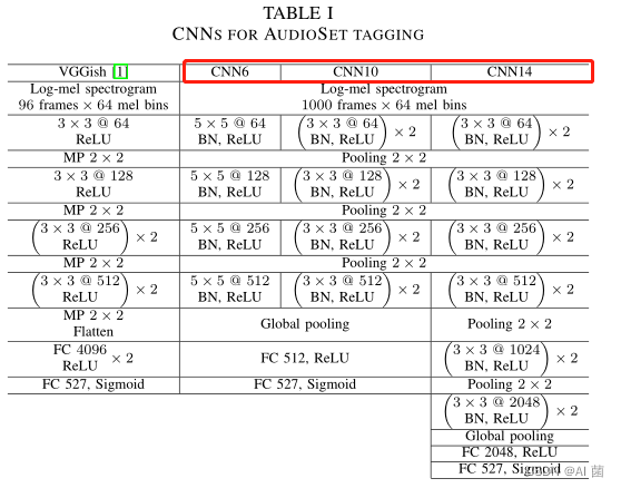
The composition of the three network architectures in the CNN series is shown below:
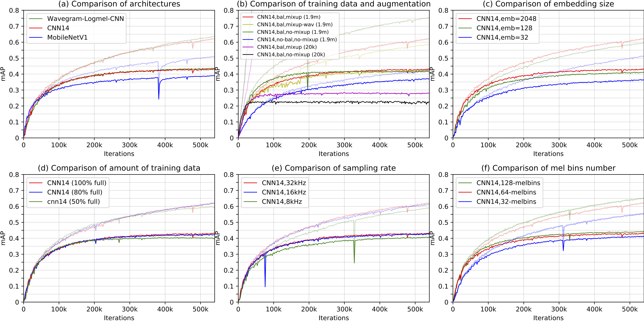
The validation metrics of different architectures in the CNN series combined with different sample rates, Mel-scale filter banks, and data augmentation strategies are shown below:
Regarding the network structure of CNN14:
- First, Mel-scale spectrograms corresponding to the audio files are generated based on
SpectrogramandLogmelFilterBankfrom thetorchlibrosalibrary. - This is followed by 6 consecutive convolutional blocks:
- The first 5 convolutional blocks consist of: 3x3 convolution + BN layer + ReLU activation function + 3x3 convolution + BN layer + ReLU activation function + 2x2 pooling layer.
- The last convolutional block consists of: 3x3 convolution + BN layer + ReLU activation function + 3x3 convolution + BN layer + ReLU activation function + 1x1 pooling layer.
- The first convolutional block outputs 64 channels, the second outputs 128 channels, and so on, with the final convolutional block outputting 2048 channels.
- The output dimension data of the final convolutional block is
[batch_size, channels, time_steps, freq_bins]. By default,channelsis 2048;time_stepsis the step size in the time dimension, which becomes 1/32 of the audio sampling frames after 5 rounds of 2x2 pooling;freq_binsrepresents frequency features, which become very small (even 1) after 5 rounds of 2x2 pooling. At this point, each time period (32 consecutive audio sampling frames) corresponds to a 2048-dimensional feature vector, which represents the fingerprint information of the sound at that moment.
- Next, global max pooling and average pooling operations are performed simultaneously on the feature vectors extracted by the continuous convolutional blocks along the time dimension, and the two are summed to obtain a 2048-dimensional feature vector.
- Finally, a fully connected layer from 2048 to
num_classesis used to perform the final classification operation based on the 2048-dimensional feature vector, yielding classification probabilities via sigmoid.