Detailed Summary of DETR (DEtection TRansformer) Network Architecture and Computational Workflow

18 Mar, 2026
- AI

This article provides a detailed introduction to the network structure and data computational workflow of DETR, an image object detection model based on the Transformer architecture proposed by Facebook in 2020.

Introduction to DETR

DETR is an AI model for object detection in computer vision proposed by Facebook AI Research (FAIR) in 2020. It introduced the Transformer architecture, widely used in the NLP domain, into computer vision for the first time. It completely revolutionized the traditional design paradigm in object detection, simplifying the task from an accumulation of tedious components and processing pipelines into a genuine end-to-end set prediction problem.

Before the advent of DETR, mainstream detectors in the object detection domain (such as Faster R-CNN, YOLO, and SSD) heavily relied on various engineering components:

Anchor Boxes: Presetting different scales and aspect ratios for detecting objects based on the overall distribution of the training dataset.
NMS (Non-Maximum Suppression): Used during post-processing to eliminate duplicate bounding boxes in the model’s output data.
Highly complex positive and negative sample matching strategies.

The core innovation of DETR lies in leveraging the global modeling capability of the Transformer structure to directly output a fixed-size set of predictions (typically 100), which are then matched one-to-one with the Ground Truth using a Bipartite Matching algorithm.

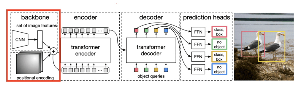
Architecturally, the DETR network mainly consists of three components: a CNN Backbone, a Transformer encoder-decoder, and a detection head.

CNN Backbone

The DETR network architecture starts with a convolutional neural network (CNN) backbone. The backbone network employs a standard ResNet (in the original paper, the authors used ResNet-50 and ResNet-101). Acting as a feature extractor for the input image, the backbone processes the raw input image to generate rich visual feature vectors.

For details on the ResNet network architecture, refer to: CNN Classical Network Architecture Learning: ResNet.

Regarding the dimensions of image processing, assuming the input image size to the backbone is $(3, H, W)$, the feature extractor processes it through multi-stage ResNet blocks to output a downscaled feature map. In a standard DETR implementation, the feature map downsampling factor is typically 32, resulting in an output feature map dimension of $(C, H/32, W/32)$. The channel dimension $C$ is usually projected to 256 using a $1 \times 1$ convolution to match the input dimension of the Transformer.

If the input image resolution is $800 \times 800$, the resolution of the output feature map will be $25 \times 25$.

Referring to the application of Transformers in computer vision within the ViT architecture (An Introduction to Vision in Transformer (ViT) Model Architecture), Transformers accept sequence data rather than matrix-form vectors. Therefore, the feature map of dimensions $(25, 25, 256)$ output by the ResNet backbone is flattened and straightened into a vector sequence of length 625, where each element is a 256-dimensional vector.

Positional Encoding

Similarly, while convolutional neural networks inherently perceive spatial information due to translation invariance and local receptive fields, Transformers process sequence data and require additional positional encoding information added to the flattened vector sequences—akin to adding positional information to text sequences in natural language processing.

DETR adopts Fixed 2D Sinusoidal Positional Encodings for the positional information of the backbone output feature map sequence. The general approach is to split the encoding information for each pixel position into $x$ and $y$ directions, encode them separately, and finally concatenate them. As mentioned above, after flattening, each pixel’s vector length is 256; hence, 128 dimensions are allocated to encode the $x$-coordinate and another 128 dimensions to encode the $y$-coordinate. Concatenating these two yields the final 256-dimensional positional feature vector.

For the $(x, y)$ coordinates of each pixel on the feature map, each $x$ corresponds to a 128-dimensional vector composed of 64 pairs of sine and cosine functions. Their calculation formulas are as follows:

$$ PE(x, 2i) = \sin\left(\frac{x}{10000^{2i/d}}\right) $$

$$ PE(x, 2i+1) = \cos\left(\frac{x}{10000^{2i/d}}\right)y $$

The 128-dimensional vector composed of 64 pairs of sine and cosine functions for the $y$-coordinate is calculated using the identical formula. The two 128-dimensional vectors are then concatenated to form a 256-dimensional positional vector. The dimension of the vector obtained in this way precisely aligns with the feature vector dimension after the $1 \times 1$ convolution, and the positional encoding information also forms a vector sequence of length 625, where each element is a 256-dimensional vector.

Transformer Encoder-Decoder

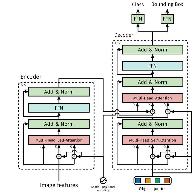
As described above, after the backbone extracts image features and flattens the feature map, the data fed into the Transformer Encoder has a dimension of a sequence of length 625, with each element in the sequence having a dimension of 256. Note that the data output by the backbone is not directly added to the positional encoding vectors; instead, the positional vectors are injected into the calculations of Query and Key during attention computation, which differs from the standard NLP Transformer computational workflow.

The figure below illustrates the processing architecture of the DETR Transformer Encoder and Decoder:

Encoder

The multi-head self-attention module of the Encoder uses 8 heads, so the dimension of each head is $d_k = 256 / 8 = 32$. The calculation of the $Q$, $K$, and $V$ matrices for each head is as follows:

Query ($Q$): $(Src + Pos) \cdot W_Q$ → Dimension: $625 \times 32$
Key ($K$): $(Src + Pos) \cdot W_K$ → Dimension: $625 \times 32$
Value ($V$): $Src \cdot W_V$ → Dimension: $625 \times 32$

Note: When calculating Queries and Keys, the feature vector $Src$ extracted by the backbone is added to its positional encoding $Pos$. The calculation of Values does not incorporate positional encodings because Values are responsible for providing content information, while $Q$ and $K$ are responsible for localization and matching.

Subsequent calculations for the multi-head attention module follow standard procedures, which are detailed in the article How to Understand Multi-Head Attention Mechanism in Transformer Architecture?.

In summary, in terms of input and output data dimensions, the flattened feature vector and positional encoding vector input to each Encoder module (the dashed box on the left of the architecture diagram above) have dimensions of $625 \times 256$, while their output data dimensions are also $625 \times 256$. The DETR model defaults to containing 6 consecutive Encoder modules, and the final output data dimension of the Encoder section remains $625 \times 256$.

The working logic of the Encoder is: Utilizing the global attention mechanism to perform context modeling on the local features extracted by the preceding backbone convolutional network, ultimately outputting an enhanced feature sequence of the same size as the input, where each point contains global contextual information and semantic features.

Decoder

To understand the architecture of the Decoder section, we first define its inputs. The input to the Decoder consists of two parts:

The output of the Encoder, which is intuitively the $625 \times 256$ tensor output by the final Encoder module.
Object Queries: A tensor of dimensions $100 \times 256$. During the training phase, these are learnable parameters (similar to embeddings). After training is complete, this $100 \times 256$ dimensional tensor serves as fixed parameters for subsequent image inference workflows. These 100 vectors represent 100 candidate bounding boxes.

As shown in the Decoder Block architecture below, each Decoder Block sequentially comprises three parts from bottom to top: a Multi-Head Self-Attention module, a Multi-Head Attention (Cross-Attention) module, and a Feed-Forward Network (FFN).

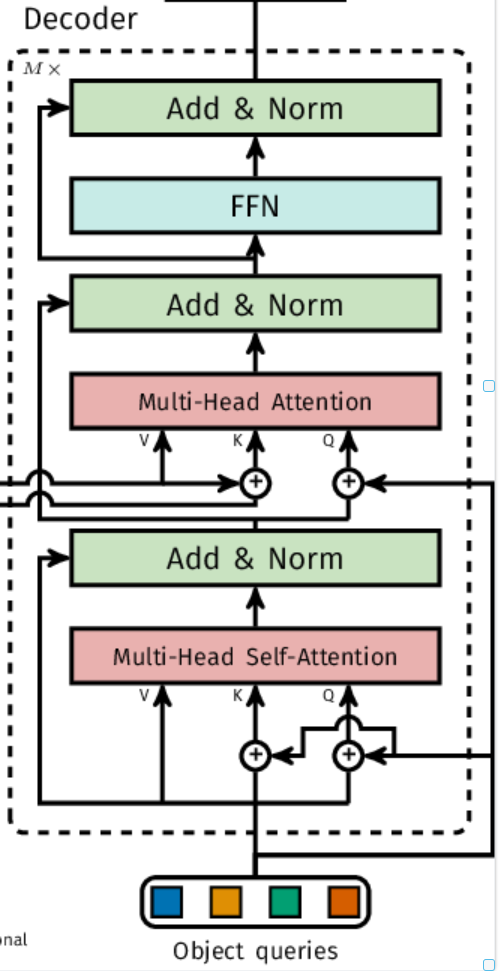
First is the self-attention module (the Multi-Head Self-Attention module in the diagram above). The computational workflow of this self-attention module differs slightly from standard Transformer self-attention: standard Transformer self-attention takes input vectors augmented with positional encoding information and multiplies them with parameter matrices $W_Q, W_K, W_V$ to obtain $Q$, $K$, and $V$ vectors; whereas the self-attention module here follows this calculation logic:

$$ V = Object_Queries \cdot W_V $$

$$ Q = (Object_Queries \oplus Object_Queries) \cdot W_Q $$

$$ K = (Object_Queries \oplus Object_Queries) \cdot W_K $$

The above self-attention calculation logic effectively uses the input Object Queries simultaneously as both input data and its positional encoding vector, which is why self-addition of Object Queries is performed during the calculation of $Q$ and $K$ in self-attention.

Why perform self-addition on the identical input Object Queries rather than multiplying the input directly by 2? This is because there are actually 6 consecutive stacked Decoder blocks. Only the first layer’s decoder uses the self-addition of Object Queries as input when calculating $Q$ and $K$; subsequent decoders use the sum of Object Queries (acting as positional vector information) and the output of the previous layer’s Decoder as their input during self-attention calculations.

After the calculation through the self-attention module above, the output data dimension is $100 \times 256$.

Next is the calculation of the Multi-Head Attention (Cross-Attention) module. In the cross-attention module, the output of the Decoder’s self-attention module acts as the active questioner, while the feature map output by the Encoder serves as the knowledge base.

The cross-attention module takes three inputs: object_queries output by the Decoder’s self-attention module (dimension $(100, 256)$), encoder_features output by the Encoder (dimension $(625, 256)$), and spatial positional encoding information identical to that of the Encoder (dimension $(625, 256)$). Under this setup, the calculation logic and data dimensions of the three tensors $Q, K, V$ are as follows:

Query ($Q$): $(Object_Queries + Query_Pos) \cdot W_Q$ → $(100, 256)$
Key ($K$): $(Encoder_Features + Spatial_Pos) \cdot W_K$ → $(625, 256)$
Value ($V$): $Encoder_Features \cdot W_V$ → $(625, 256)$

The subsequent calculation logic of the cross-attention module and the feed-forward network (FFN) module remains identical to the standard Decoder Block workflow (refer to A Comprehensive Guide to the Decoder Structure and Computational Workflow of the Transformer Model for details). Ultimately, the output dimension of the entire Decoder Block is identical to its input dimension, both being $(100, 256)$. The Decoder section on the right side of the DETR network structure contains a total of 6 consecutive stacked Decoder blocks, where the output of each block serves as the object queries input for the next block. Thus, the final output data dimension of the entire Decoder section remains $(100, 256)$.

Detection Head

As mentioned above, after continuous stacking and processing through the 6 Decoder blocks of the entire Decoder section, the final output data dimension of the Decoder is $(100, 256)$. The task of the final detection head in the DETR model is to map these 100 high-dimensional vectors into human-readable class labels and bounding box coordinates.

For the design of the detection head structure, DETR adopts two parallel FFN (Feed-Forward Network) branches that share the Decoder’s output but handle distinct tasks.

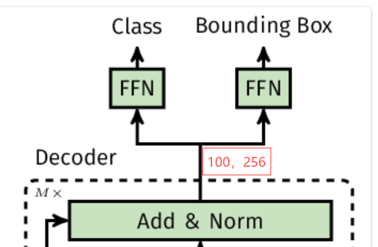
The Classification Head structure is a simple Linear Layer. The input data dimension of this linear layer is $100 \times 256$, and the output data is $100 \times (K+1)$, where $K$ is the number of target dataset classes (such as 80 classes in COCO), and $+1$ represents the background class (no object). The final activation function uses Softmax, which assigns a probability distribution to each query, indicating which class the object corresponding to that query belongs to.

The Bounding Box Regression Head structure is a Multi-Layer Perceptron (MLP) with 3 hidden layers, each interspersed with a ReLU activation function. The input data dimension for the entire regression head is $100 \times 256$, and the output data dimension is $100 \times 4$. The numerical values represent the normalized center coordinates, width, and height: $(x_{center}, y_{center}, w, h)$.

With the above output head structure, for each image, the DETR model outputs coordinate information for 100 bounding boxes (from the regression head), with each bounding box corresponding to classification information of length $K+1$. When filtering background boxes, one simply needs to set a threshold (e.g., 0.5) to filter out prediction boxes whose classification result is the background class (no object) or whose scores are too low, thereby eliminating the need for the extremely complex NMS computation pipeline found in models like YOLO.