A Beginner's Guide to the Vision Transformer (ViT) Model Architecture
- 25 Feb, 2026
This article provides a detailed summary of the Vision Transformer (ViT) model architecture and the complete image processing workflow within it, helping to build a foundational understanding of the ViT model.
While the Transformer architecture has been widely adopted across various Large Language Models in Natural Language Processing (NLP), Google’s milestone 2020 paper “An Image is Worth 16×16 Words” introduced the Transformer to computer vision. By leveraging Patch Embedding and self-attention mechanisms, it has profoundly challenged the traditional dominance of Convolutional Neural Networks (CNNs) in computer vision, signaling a unifying trend across all domains of artificial intelligence.
To understand the ViT model architecture and how image data is processed within it, you first need a clear understanding of the Transformer architecture, especially its Encoder section. You can refer to another related note: [[一文彻底搞懂Transformer模型的Encoder结构与计算流程]].
Introduction to the ViT Architecture
The Transformer architecture was originally designed for sequential data (1D), whereas images are high-dimensional (Width $\times$ Height $\times$ Channels). When feeding image data into a Transformer, the first challenge is converting high-dimensional image data into a 1D sequence that the Transformer can accept. The most intuitive approach would be to treat every individual pixel in the image as a token fed into the model, but this results in an exponential explosion in computational complexity. Therefore, ViT’s solution is: patch the image and serialize the resulting patches as inputs to the Transformer model.
In essence, the ViT model splits the input image into a sequence of fixed-size patches, serializes these patches, and applies the Transformer’s self-attention mechanism to extract image features. This enables the model to capture long-range dependencies between different parts of the image without relying on CNN convolution operations.
The figure below illustrates an image classification model based on the ViT architecture. As shown, the input image is divided into multiple fixed-size patches, which are then serialized and vectorized before being fed into the Transformer Encoder for feature extraction. Finally, classification results are output through an MLP Head. Structurally, compared to the Transformer Encoder used for natural language semantic extraction, the only major difference in ViT is the patch-slicing preprocessing applied to the image.
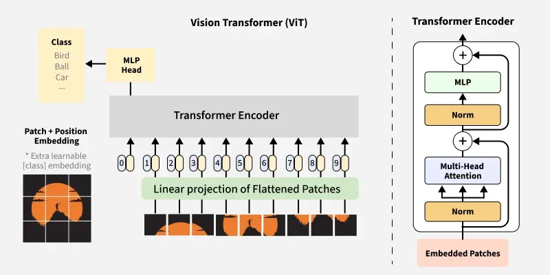
The processing workflow of the ViT-based image classification model can be broken down into several steps, which are analyzed and described below.
1. Image Patching
This step is conceptually similar to tokenization and embedding operations performed on text sentences and paragraphs in NLP pipelines.
First, the image undergoes a patching operation. For example, if a 224 × 224 image is divided into fixed-size 16 × 16 blocks (where each block is a patch), the entire image will be split into $14 \times 14 = 196$ patches.
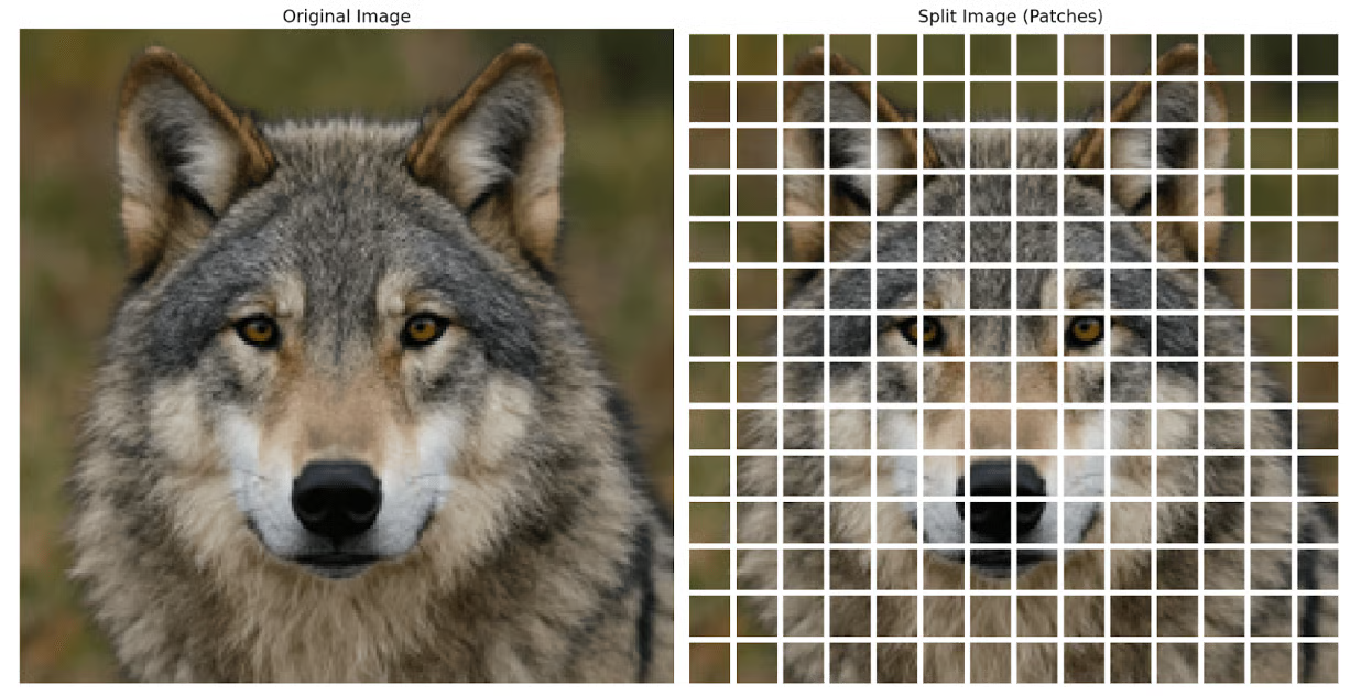
Since each input image typically contains three RGB channels, the dimensions of each sliced patch are $16 \times 16 \times 3$. This patch remains a 3D tensor, whereas the Transformer’s self-attention mechanism operates on fixed-length 1D vectors. Therefore, the next step requires flattening this $3D$ tensor ($16 \times 16 \times 3$) into a 1D vector.
In practical engineering implementations, slicing the input image and flattening each patch are typically performed using a 2D convolution layer whose stride equals its kernel size. For instance, with a patch size of $16 \times 16$ and an output 1D vector length of 768 per flattened patch, you can use the following 2D convolution operation to execute both patching and flattening:
Conv2d(in_chans=3, out_chans=768, kernel_size=16, stride=16)Because the kernel size matches the patch size precisely, a single convolution step extracts the features of one patch, which yields higher computational efficiency on GPUs.
Through these operations, an input image with a resolution of $224 \times 224$ is divided into 196 patches, with each patch flattened and mapped into a 1D vector of length 768.
2. Adding the Cls Token
Before further processing the 196 patch vectors obtained above, an additional classification vector of the same length (768), known as the Cls Token, is appended. This classification token does not represent any specific image patch; its sole task is to interact with the other 196 patches, allowing the final classification result for the entire image to be read from its output representation.
Specifically, a learnable vector of shape (1, 768) is manually created and prepended to the front of the 196 patch vectors. Following this step, the input sequence length becomes $196 + 1 = 197$ vectors, with each vector having a length of 768.
3. Positional Encoding
The subsequent process follows the same logical flow as natural language text sequences: positional encoding is added to the 197 vectors to preserve the spatial awareness of each patch’s location within the original input image. Just as word positions are critical for understanding semantic meaning in natural language sequences, the spatial location of each patch is vital for extracting comprehensive image features. Consequently, explicit positional information must be added to these vector sequences before feeding them into the Transformer.
The dimensions of the positional encoding matrix match the input matrix shape (e.g., $197 \times 768$) precisely, and this step is accomplished by directly adding the positional embedding matrix to the preceding patch vector matrix.
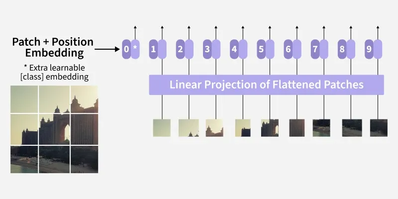
At this point, after undergoing the aforementioned processing steps, the input image data is fully prepared to enter the Transformer Encoder for self-attention computation. A $224 \times 224$ resolution image has been transformed into a sequence of shape (197, 768) enhanced with positional encodings.
4. Transformer Encoder
The processing logic and workflow within the Transformer Encoder are identical to those used for natural language text. The entire Transformer Encoder consists of a consecutive stack of $L$ identical Encoder Blocks:
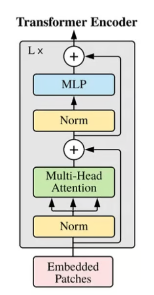
Each Transformer Block contains structures such as Multi-Head Attention modules, Feed-Forward Networks (FFN), and Residual Connections with Layer Normalization. The working logic and calculation workflow of the entire Transformer Encoder can be found in [[一文彻底搞懂Transformer模型的Encoder结构与计算流程]], while the calculation workflow of its Multi-Head Attention module can be referenced in [[如何理解Transformer架构中的多头注意力机制?]].
The input and output tensor dimensions of each Encoder remain unchanged. Therefore, after passing through all Encoder layers, the output is still a matrix of shape (197, 768).
5. MLP Head (Classification Head)
As described above, the output of the Transformer Encoder module is a (197, 768) matrix containing the fully extracted feature information of the input image. For classification tasks, however, we only need to extract the CLS Token vector at index 0 (i.e., the extra vector appended during the second step).
For image classification tasks, the role of the classification head is essentially information compression and mapping: translating the highly abstract 768-dimensional feature vector into class probability predictions. Therefore, the classification head of a ViT model typically consists of a simple Multi-Layer Perceptron (MLP). For instance, a standard classification head network structure comprises two linear layers sandwiching an activation function to enhance non-linear mapping capabilities, concluded with a Softmax layer to generate probabilities:
- Slice and extract the vector at index 0 from the
(197, 768)output matrix of the Transformer Encoder. - Linear layer
(768 → 768) - Tanh or GELU activation function
- Linear layer
(768 → K), where $K$ is the number of classes - Softmax
Testing a Pre-trained ViT Image Classification Model
The following code uses Hugging Face’s Transformers library to download a pre-trained image classification model based on the ViT architecture and performs forward inference to obtain the final result:
from transformers import ViTImageProcessor, ViTForImageClassification
from PIL import Image
import torch
import requests

image = Image.open('D:/test/cats+dogs/images/dog.jpg')

processor = ViTImageProcessor.from_pretrained('google/vit-base-patch16-224')
model = ViTForImageClassification.from_pretrained('google/vit-base-patch16-224')

# Preprocessing the image so it gets it into the necessary format
inputs = processor(images=image, return_tensors='pt')

# Forward pass - with no backpropagation
with torch.no_grad():
    outputs = model(**inputs)

    logits = outputs.logits
    predicted_class = logits.argmax(-1)

    id2label = model.config.id2label
    predicted_label = id2label[predicted_class.item()]
    print(f"Predicted class index: {predicted_class.item()}")
    print(f"Predicted class label: {predicted_label}")
Where:
ViTImageProcessoris used to preprocess the input image, including resizing and normalization, ultimately converting the raw image into a format acceptable to the ViT model. This preprocessing routine is somewhat analogous to the tokenization process applied to natural language text before Transformer processing.ViTForImageClassificationis the actual ViT classification model. It receives the image tensor output preprocessed byViTImageProcessorand outputs the classification logits. Consequently, a Softmax function must ultimately be applied independently to obtain the classification probabilities.