How to Understand Multi-Head Attention in the Transformer Architecture?

Introduction to the Self-Attention Mechanism

The self-attention mechanism in the Transformer model was first introduced in the 2017 paper “Attention is All You Need” by Google AI researchers. It quickly became the core concept of the Transformer model, which in turn forms the foundation of various Large Language Models (LLMs) and Vision Language Models (VLMs). The brilliance of the self-attention mechanism lies in granting the model a global field of view: it allows every pixel (or feature point) in an image to directly connect with every other pixel (ViT), and every word (Token) in a serialized natural language paragraph to directly connect with all other words in the entire paragraph (LLM).

Consider the following example to illustrate this:

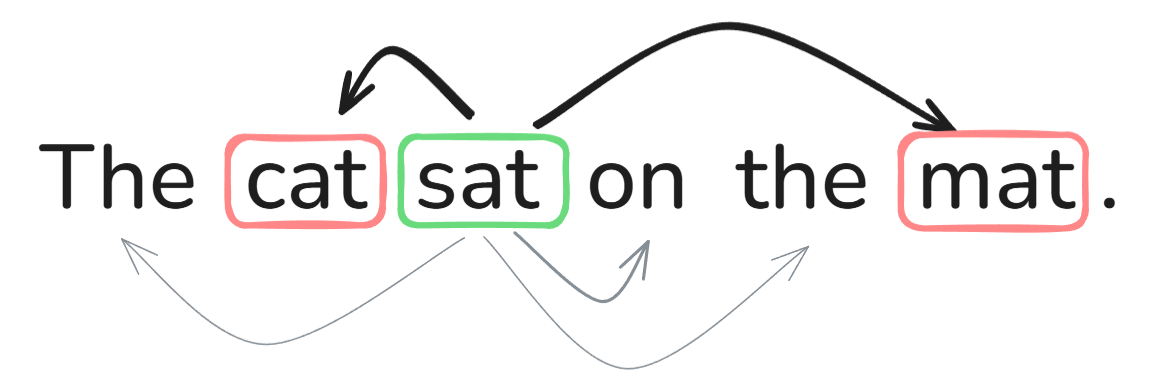
When trying to understand this simple sentence, upon seeing the word “sat”, our attention naturally focuses on the closely related words “cat” and “mat”, while other words hold little significance for understanding “sat” and can basically be ignored. Therefore, so-called attention means: based on semantic or grammatical relationships, helping the model determine the relevance and closeness between other words in the text and the word currently being processed. The closer the relationship between two words, the higher their weight; otherwise, the lower their weight.

Preprocessing

Of course, before performing self-attention computations, the serialized text data must first be preprocessed. For text data, the preprocessing pipeline mainly consists of three parts:

• Tokenization: Breaking down the paragraph and sentences semantically into individual, independent words (tokens).
• Embedding: Vectorizing the tokens generated above. Roughly speaking, this is like looking up a dictionary to map each token to a fixed-length vector.
• Positional Embedding: Additionally, a positional encoding of the same length is added to each token’s vector. This positional encoding reflects the token’s position within the entire paragraph or sentence.

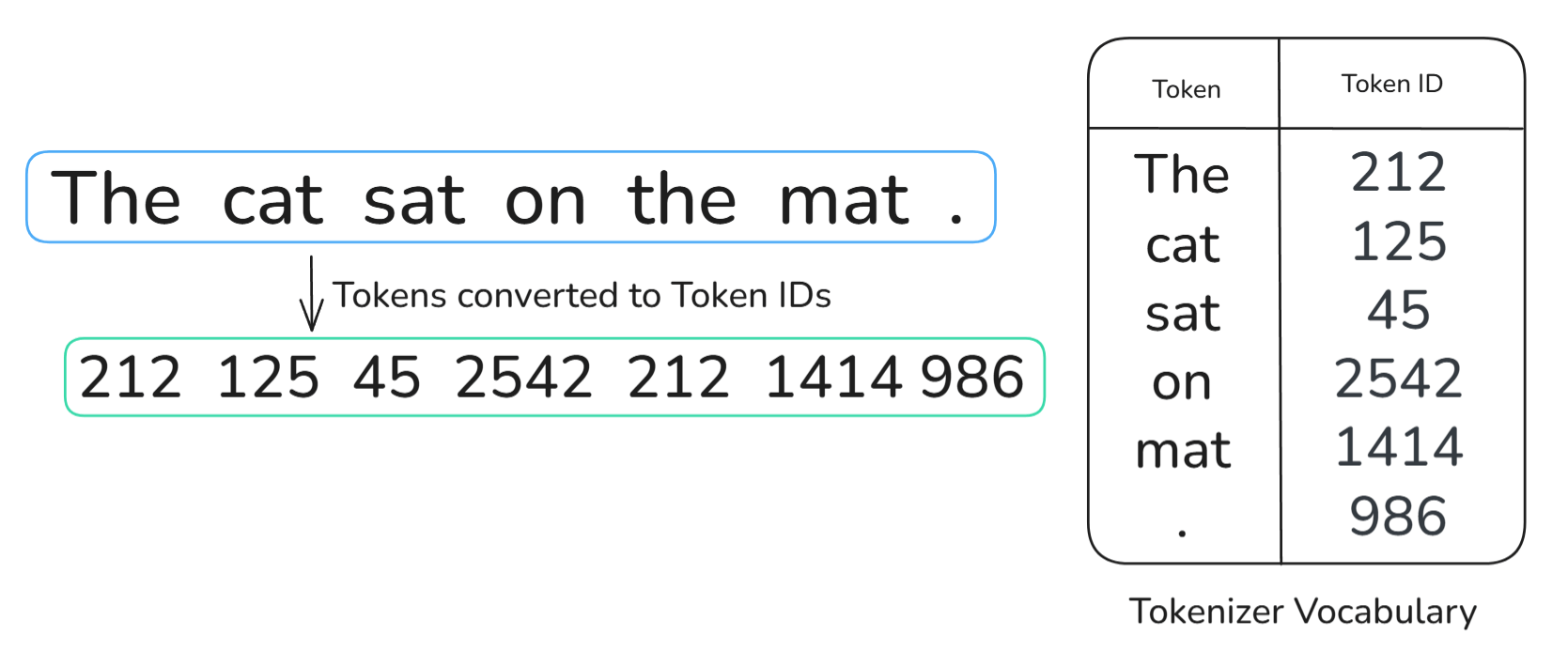
At this point, the serialized text of the entire paragraph has been converted into individual tokens, with each token corresponding to a fixed-length vector (e.g., 512, 768) enriched with positional encoding information. These vectors serve as the input data for the subsequent self-attention computation.

Q, K, V Matrices

The core design of the self-attention mechanism is transforming the input vector into three distinct roles: Query ($Q$), Key ($K$), and Value ($V$).

We can use a search engine as an analogy for these three roles:

• Query ($Q$): The “keywords” you type into the search box (“What am I looking for?”).
• Key ($K$): The “titles/tags” of videos in the database (“What features do I have to be matched against?”).
• Value ($V$): The actual “video content” corresponding to the search results (“What information can I provide if matched?”).

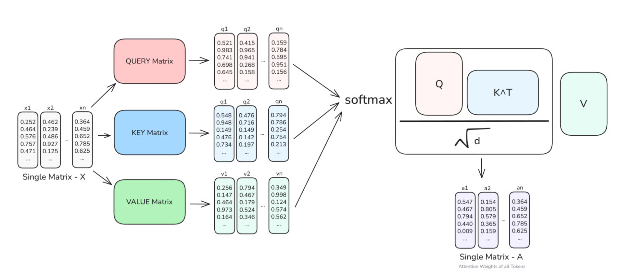
From the perspective of mathematical operations, the first step of self-attention computation takes the vectors produced by the aforementioned serialized data as input, and multiplies them separately by three weight matrices $W^Q, W^K, W^V$ to yield the $Q, K, V$ vectors.

Suppose the input paragraph is tokenized into 64 tokens, and the vector length for each token is 512. Then the dimension of the input data is $(64, 512)$, and the dimensions of the three weight matrices $W^Q, W^K, W^V$ are all $(512, 512)$. Consequently, the resulting $Q, K, V$ vectors have the same dimension as the input data, which remains $(64, 512)$.

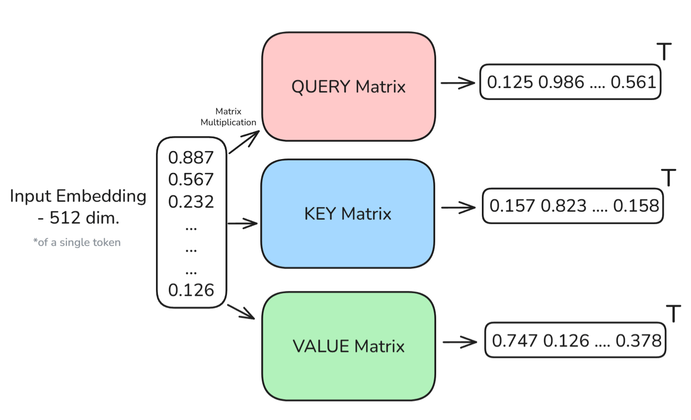
For the input vector of each token, the QSK calculations are performed separately to obtain three corresponding Q, S, and K vectors. Then, while processing each token, its similarity with other tokens (including itself) is computed through the dot product of its own $Q$ vector and the $K$ vectors of other tokens, thereby measuring the correlation between two elements as $QK^T$.

For example, taking the sentence above, we use the query vector $Q$ of “sat” and compute it against the key vectors $K$ of every other word in the sentence (including “sat” itself). The result is a set of similarity scores (which are scalars) telling us how relevant each word is to “sat”, and these scores are what we call attention scores.

To prevent the calculated attention scores from suffering from vanishing or exploding gradients, they are divided by a scaling factor $\sqrt{d_k}$ (where $d_k$ is the feature dimension, e.g., 512). Then, they are converted into a probability distribution via Softmax (where the sum of weights equals 1), and these weights are ultimately multiplied by $V$ to produce the final output.

$$ \text{Attention}(Q, K, V) = \text{softmax}\left(\frac{QK^T}{\sqrt{d_k}}\right)V $$

Through this complex calculation process, we finally obtain a new vector representation for the word “sat” in its current context. This new vector information comprehensively considers the semantics of all words in the entire sentence, though it is primarily derived from related tokens like “cat” and “mat”.

This calculation process is executed for every token in the sentence. The semantic extraction of each token simultaneously attends to all other tokens, and even to itself—which is why we call it the self-attention mechanism.

How Do the Attention Formulas Reflect the Relationships of Q, K, and V Matrices?

As mentioned earlier when explaining the $Q, K, V$ vectors:

• $Q$ is the Query, representing the specific semantics the current token wants to query from all tokens contained in the paragraph.
• $K$ is the Key, representing the list of features possessed by all tokens in the paragraph.
• $V$ is the Value, representing the auxiliary semantics that other tokens can provide to the current token when $Q$ and $K$ match.

The computational formula for the QKV matrices is:

$$ \text{Attention}(Q, K, V) = \text{softmax}\left(\frac{QK^T}{\sqrt{d_k}}\right)V $$

So how do these two aspects establish a connection?

In the formula above, the first step is to compute $QK^T$. When taking the dot product of the $Q$ vector (“What am I looking for?”) and the $K$ vector (“What features do I have?”), it essentially calculates: “How well does the requirement described by the current Query match the attributes provided by this Key?” From the perspective of matrix computation, let $N$ be the total number of tokens in the text paragraph, and $d_k$ be the vector length of each token (e.g., 512, 768). Then, the $Q$ matrix corresponding to all tokens in the paragraph is of size $N \times d_k$, the $T$ transpose of $K$ ($K^T$) is of size $d_k \times N$, and the resulting multiplied $QK^T$ matrix for all tokens has a size of $N \times N$ (this result is actually the attention score matrix among all tokens). Each row represents the matching score table of a specific token against all tokens in the paragraph for precise semantic parsing.

The scores calculated via the dot product above can be any real numbers and cannot be used directly to aggregate information. This is where Softmax comes in: Softmax amplifies high scores, suppresses low scores, and then normalizes them, transforming all scores into probabilities between 0 and 1 that sum up to 1.

The final step is to multiply the attention score matrix processed above with the $V$ vectors of all tokens. Mathematically, this is a weighted summation process. Its output is a new feature vector filtered by weights (where the weights are the attention score matrix) that encapsulates the contextual information of the entire paragraph.

In summary, the essence of the $Q, K, V$ vectors and their attention formula is to extract the precise semantics that the current token represents within the paragraph. The specific calculation process involves first computing the matching degree between the current token’s $Q$ vector and the $K$ vectors of all tokens in the paragraph (including the current token itself). The result reflects the relative importance (i.e., attention scores) of all tokens in the paragraph when parsing the precise semantics of the current token. Then, based on this importance, the $V$ vectors of all tokens are extracted, and their weighted sum yields the precise semantics of the current token in the current paragraph.

With this, the logical concepts and complete computational flow of the self-attention mechanism have been explained.

Why Multi-Head?

Now let us consider a question: If we only use a single set of $Q, K, V$ (single head), the current token can only extract semantics from a single dimension at a time. However, in complex text semantic processing, a single token element may possess multiple relationships across different dimensions.

Example: “Xiao Ming borrowed a thick book from the library.” When extracting the precise semantics of the word “book”, multiple distinct dimensions are involved:

• Grammatical aspect: Attending to “borrowed”, identifying that “book” is the object of the verb.
• Attributive aspect: Attending to “thick”, extracting the physical characteristics of the “book”.
• Locational aspect: Attending to “library”, extracting the scenario where the action takes place.

Therefore, if there is only a single head, the model is forced to encode grammatical, attributive, and locational scenario information simultaneously within the exact same set of $Q, K, V$ weights. This dilutes the attention, making it difficult for the model to capture these multi-dimensional features accurately and concurrently. The introduction of the multi-head mechanism allows the model to independently learn these multi-dimensional relationships across different subspaces.

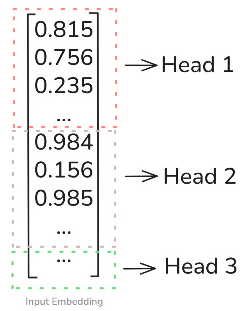
The operational and computational flow of multi-head attention is actually quite straightforward. The computation steps are identical to the single-head attention mechanism described above, except that the input feature vectors are split into multiple sub-vectors of equal length:

• Split: The high-dimensional input feature vector (e.g., 512 dimensions) is split into multiple lower-dimensional sub-vectors (e.g., 8 heads, making each head 64 dimensions).
• Parallelism: The 8 split heads independently and in parallel perform the aforementioned $Q, K, V$ computations.
• Concat: The computation outputs from each of the 8 heads (each 64 dimensions) are concatenated back together into a 512-dimensional long vector.
• Linear: Finally, it is multiplied by a weight matrix $W^O$ to perform a final fusion processing of these multi-dimensional computation results.

References

• Understanding Multi-Head Attention in Transformers | DataCamp
• What is Attention and Why Do LLMs and Transformers Need It? | DataCamp