A Comprehensive Guide to Understanding the Encoder Structure and Computation Workflow of the Transformer Model

22 Feb, 2026
- AI

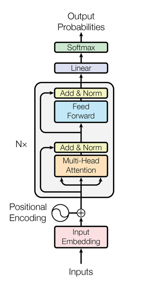
The diagram below illustrates a standard Encoder-Only Transformer architecture:

In general, the execution workflow of an Encoder-Only Transformer architecture proceeds in the following sequence:

Data preprocessing phase, which includes input data vectorization (Embedding) and the addition of positional encodings.
A sequential stack of $N$ Encoder Blocks.
The data output phase.

For an Encoder-Only Transformer architecture, the data output phase is very straightforward—such as the Linear + Softmax output shown in the figure above. Therefore, the focus of this article will be on the computation workflows of the first two parts.

1. Data Preprocessing

For Natural Language Processing (NLP) Transformer architectures, data must undergo at least the following steps before entering the Encoder and Decoder of the Transformer:

Tokenization: Breaking down a complete sentence or paragraph into independent semantic units, known as tokens. This step can be accomplished using currently available, highly efficient tokenization tools.
Embedding: Based on the tokenization results, each independent token is converted into a vector of a fixed length (e.g., 512, 768, etc.). After this vectorization step, each token corresponds to a vector of uniform length.
- Taking a vector length of 768 as an example, if the text to be processed contains 100 tokens, it will be converted into a tensor of shape (100, 768) after this step.
Positional Encoding: Adding positional encoding to the vectorized tokens from the previous step. The length of the positional encoding matches the token’s vector length, so each token’s vector can be directly added to its corresponding positional encoding vector without changing the data dimensions.
- Continuing with the previous (100, 768) vector example, the dimensions remain (100, 768) after adding the positional encodings.

The diagram below illustrates the complete data preprocessing workflow for the text “How are You”:

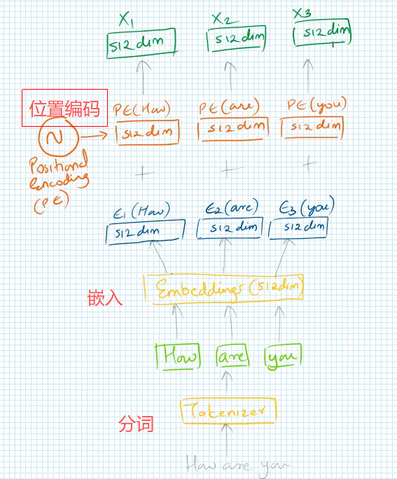
Following the data preprocessing stage, a piece of text (split into $N$ tokens, where each token has a vector length of dimension) is transformed into a tensor of shape (N, dimension), ready for the Encoder processing stage.

2.1 Q, K, and V Matrices in Multi-Head Attention

As is well known, the core of the Transformer is the Self-Attention mechanism, whose working logic computes the correlation between each element and all other elements in the input sequence. The key components of this self-attention mechanism are $Q$, $K$, and $V$. Self-attention can be conceptualized as an “information retrieval” process:

Query (Q): What am I looking for? (Features of the current patch/element)
Key (K): What do I have? (Feature tags of all other patches/elements)
Value (V): What can I provide? (The actual content information)

Just looking at the definitions above might not feel entirely intuitive. How exactly do these $Q$, $K$, and $V$ function within the data processing workflow? To state the conclusion directly: If the vector length of each token is dimension, then $Q$, $K$, and $V$ are three independent weight parameter matrices of shape (dimension, dimension). These three weight matrices are the parameters to be trained during the training process.

Assuming a token vector $x$ has a dimension of $1 \times d$, then $W_Q, W_K, W_V$ are three matrices of dimension $(d, d)$. The computation process for $Q$, $K$, and $V$ with respect to this token vector $x$ simply multiplies the token vector by each of the three parameter matrices, mapping the input token vector into a new space:

$$ \begin{aligned} q = x \cdot W_Q \ k = x \cdot W_K \ v = x \cdot W_V
\end{aligned} $$

As shown in the figure below: The text “Data visualization empowers users to” is split into 6 tokens, and the vector length for each word is 768. In this case, the dimension of each token is (1, 768), while the dimensions of the three weight matrices $W_Q, W_K, W_V$ are each (768, 768). Combined, the dimension of the three matrices together is (768, 2304).

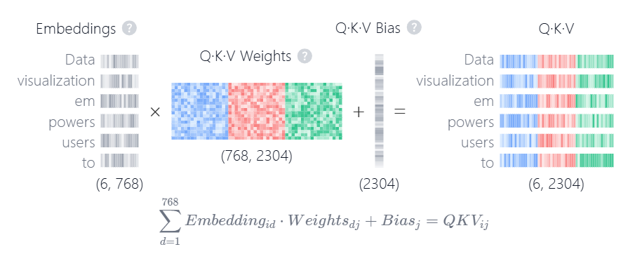
In summary, during this step, the (1, dimension) vector corresponding to each token is transformed via the above computation into three independent (1, dimension) vectors, corresponding to the token’s $Q$, $K$, and $V$ vectors respectively. The combined dimension of these three sets of vectors is (1, 3 x dimension).

2.2 Attention Computation Workflow in Multi-Head Attention

After the processing in the previous step, we obtain the $Q$, $K$, and $V$ vectors for all words in a text sequence. The next computation step is to extract the corresponding $V$ vectors based on the $Q$ and $K$ vectors.

First, compute the dot product between the $Q$ vectors and $K$ vectors for all tokens in the text sequence. This measures the degree of attention that the $i$-th token pays to the $j$-th token:

$$ Score_{i,j} = Q_i \cdot K_j^T $$

The closer the vector directions of $Q_i$ and $K_j$, the higher the calculated score. After this computation (assuming the text contains $N$ tokens), the resulting score matrix has a dimension of (N, N).

To prevent exploding gradients from the above computation and to convert the results into probabilities, two additional steps are required:

Scaling: Divide each score above by $\sqrt{d_k}$. Here, $d_k$ is a scaling factor that ensures the model remains stable during training even when stacked deeply. For a designed Transformer model, $d_k$ is a constant, typically equal to the data dimension divided by the number of heads.
Softmax: Transform the score matrix into a weight matrix $\alpha_{i,j}$ ranging between $0$ and $1$.

$$ \alpha_{i,j} = \text{softmax}\left(\frac{Q_i K_j^T}{\sqrt{d_k}}\right) $$

The computation workflow for these two steps is highlighted by the red box in the diagram below: The matrix $\alpha_{i,j}$ processed by softmax still has a dimension of (N, N). In the illustration below, the text contains only 6 tokens, so this matrix has a dimension of (6, 6).

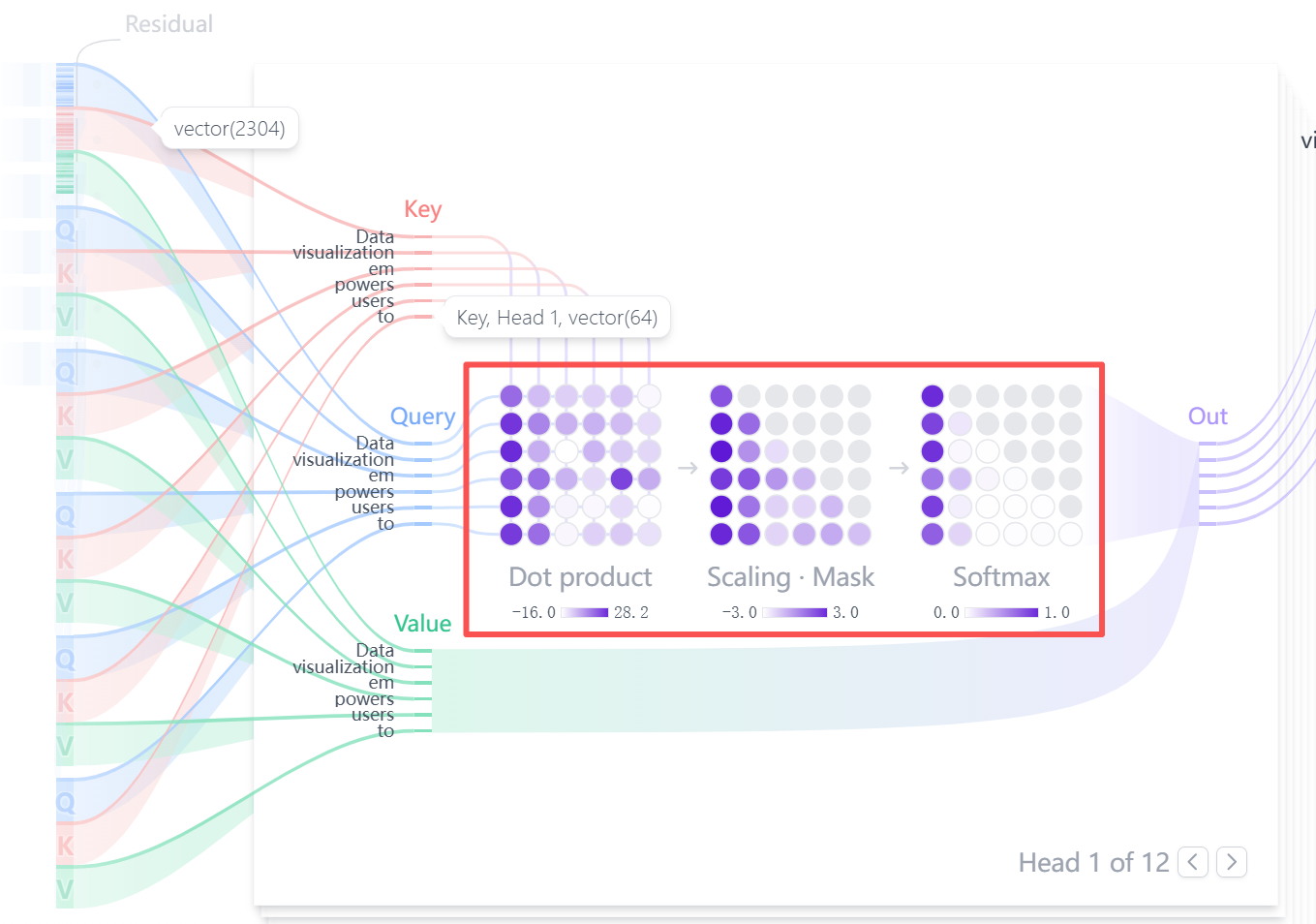
With the weight matrix $\alpha_{i,j}$ obtained above, we can use it to aggregate all the Values (i.e., the $V$ matrix):

$$ \text{Output}i = \sum{j} \alpha_{i,j} V_j $$

As shown in the red box of the diagram below: Assuming the text contains $N$ tokens and each token has a vector length of dimension, this computation is the product of an (N x N) dimensional matrix (the weight matrix calculated from $Q$ and $K$) and an (N x dimension) dimensional matrix. The final output structure remains (N x dimension).

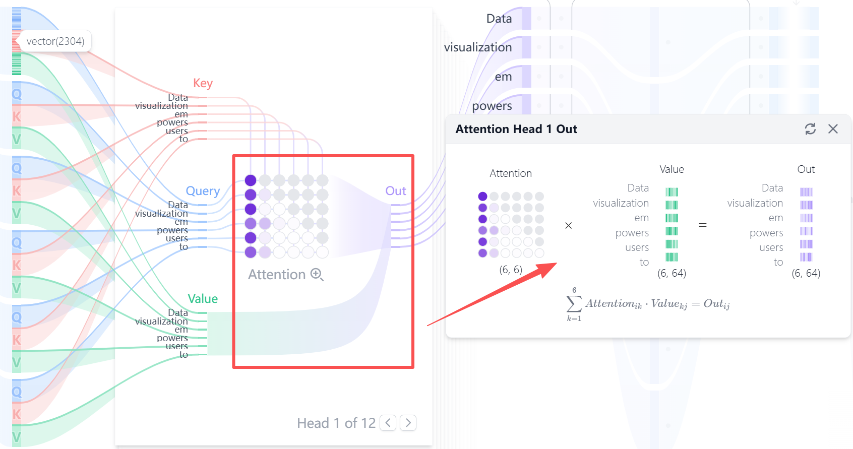
At this point, the computation workflow for the self-attention $Q$, $K$, and $V$ matrices in the Encoder module is complete. The entire Encoder computation takes data of shape (N, dimension) as input and yields an output of shape (N, dimension), meaning the data dimensions remain unchanged.

Wait! There is another question: Earlier, during the Embedding transformation process for individual tokens, it was explicitly mentioned that each token’s vector length is 768. However, during the final $V$ matrix operation above, it is clearly visible that the dimension of the $V$ matrix is (6, 64) instead of (6, 768), and the final output is also (6, 64) rather than (6, 768). This brings up the concept of Multi-Head.

2.3 Multi-Head in Multi-Head Attention

Let us examine the complete block diagram of the Multi-Head Self-Attention Block: On the left are the $Q$, $K$, and $V$ matrices for all input tokens, with a data dimension of (N, 3 x dimension); on the right is the processing result of this multi-head attention module, with a dimension of (N, dimension).

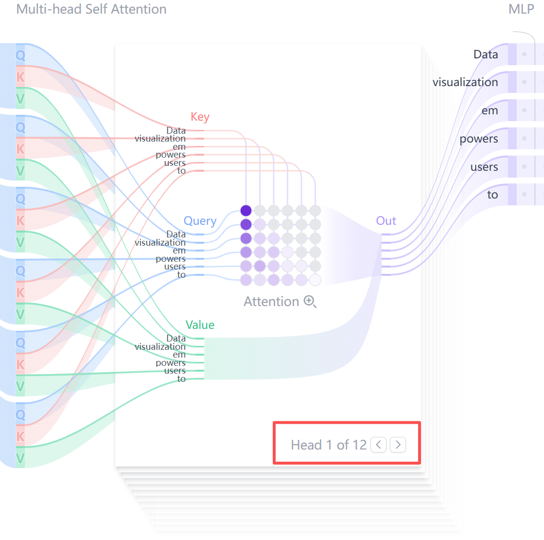
The red-boxed notation below indicates that the operations of the entire attention module are divided into 12 independent, parallel computing modules executed simultaneously, after which the results are merged. This is what is known as multi-head attention.

For example, in the figure above, there are 6 tokens, and the data dimension for each token is 768. Therefore, for the entire self-attention module, the input consists of three independent (6, 768) matrices—namely the respective $Q$, $K$, and $V$ vectors for the 6 tokens. In the multi-head processing setup, the computation workflow splits into 12 heads, dividing the input data into 12 independent groups. For each token’s $Q$, $K$, and $V$ vectors, each vector of length 768 is split into 12 segments, where each segment has a length of $768 / 12 = 64$ (which explains the 64 appearing in the $V$ matrix calculation above). Thus, for the computation of each head, the input data dimension becomes three independent (6, 64) matrices (for the $Q$, $K$, and $V$ vectors), the output data dimension for a single head is also (6, 64), and all head outputs are concatenated back together to form (6, 768).

This is the essence of multi-head attention: splitting the input $Q$, $K$, and $V$ vectors of each token into $N$ equal parts, processing these $N$ parts simultaneously, and then merging them. The final input and output data dimensions remain consistent.

You can refer to the code snippet below for a deeper understanding of the working mechanism of the multi-head self-attention module:

class MultiHeadAttention(nn.Module):
    def __init__(self, embed_dim, num_heads):
        super().__init__()
        self.num_heads = num_heads
        self.head_dim = embed_dim // num_heads
        assert embed_dim % num_heads == 0, "embed_dim must be divisible by num_heads"
        # Weight calculation and parameter matrices for Q, K, V vectors
        self.q_linear = nn.Linear(embed_dim, embed_dim)
        self.k_linear = nn.Linear(embed_dim, embed_dim)
        self.v_linear = nn.Linear(embed_dim, embed_dim)
        self.out_linear = nn.Linear(embed_dim, embed_dim)

    def forward(self, query, key, value, mask=None):
        batch_size = query.size(0)
        # Q, K, V vector computations
        Q = self.q_linear(query).view(batch_size, -1, self.num_heads, self.head_dim).transpose(1, 2)
        K = self.k_linear(key).view(batch_size, -1, self.num_heads, self.head_dim).transpose(1, 2)
        V = self.v_linear(value).view(batch_size, -1, self.num_heads, self.head_dim).transpose(1, 2)
        # Compute score matrix based on Q and K vectors
        scores = torch.matmul(Q, K.transpose(-2, -1)) / math.sqrt(self.head_dim)
        if mask is not None:
            scores = scores.masked_fill(mask == 0, float('-inf'))
        # Softmax processing of the score matrix
        attention_weights = torch.softmax(scores, dim=-1)
        # Fusion computation between the score matrix and V vector
        attended_output = torch.matmul(attention_weights, V)
        # Concatenate multi-head output data
        attended_output = attended_output.transpose(1, 2).contiguous().view(batch_size, -1, self.num_heads * self.head_dim)
        output = self.out_linear(attended_output)
        return output

3.0 Feed Forward

The feed-forward network in the Encoder module is relatively simple. It is essentially implemented by sandwiching a non-linear activation function between two linear layers to achieve non-linear transformation of the output data, while keeping the input and output data dimensions as (N, dimension):

class PositionwiseFeedForward(nn.Module):
    def __init__(self, embed_dim, ff_dim):
        super().__init__()
        self.linear1 = nn.Linear(embed_dim, ff_dim)
        self.relu = nn.ReLU()
        self.linear2 = nn.Linear(ff_dim, embed_dim)

    def forward(self, x):
        return self.linear2(self.relu(self.linear1(x)))

4.0 The Complete Encoder Block

The block diagram of a complete Encoder Block is shown below:

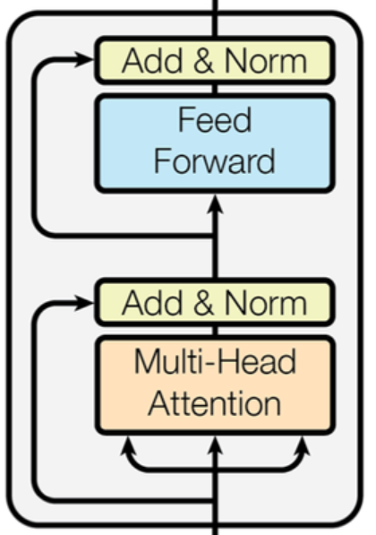
As can be seen, an independent encoder block is essentially a multi-head attention module with its residual connection, followed by a feed-forward network module with its residual connection. Given our understanding of the multi-head attention and feed-forward modules above, comprehending the execution workflow of the encoder block below becomes quite straightforward:

class EncoderLayer(nn.Module):
    def __init__(self, embed_dim, num_heads, ff_dim, dropout_rate):
        super().__init__()
        self.self_attn = MultiHeadAttention(embed_dim, num_heads) # Multi-head attention module
        self.feed_forward = PositionwiseFeedForward(embed_dim, ff_dim) # Feed-forward network module
        self.norm1 = nn.LayerNorm(embed_dim)
        self.norm2 = nn.LayerNorm(embed_dim)
        self.dropout = nn.Dropout(dropout_rate)

    def forward(self, x, mask=None):
	    # Multi-head attention module computation
        attn_output = self.self_attn(x, x, x, mask)
        # Residual connection and layer normalization for the multi-head attention module
        x = self.norm1(x + self.dropout(attn_output))
        # Forward computation of the feed-forward network module
        ff_output = self.feed_forward(x)
        # Residual connection and layer normalization for the feed-forward network module
        x = self.norm2(x + self.dropout(ff_output))
        return x

At this point, the complete computation workflow for a single Encoder Block is established. Note that for a single encoder block, both the input and output data dimensions are identical—namely (N, dimension)—making it easy to stack multiple encoder blocks sequentially to form the complete Transformer architecture.

5.0 The Complete Transformer Encoder Architecture

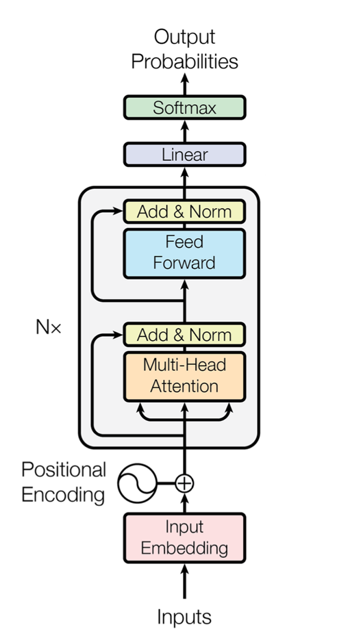
Revisiting the complete Transformer encoder architecture, it becomes very easy to understand:

First is the data preprocessing part. Input text and other sequence data undergo tokenization and vectorization to convert each token into a fixed-length vector, which is then combined with positional encoding to produce position-encoded vectors of uniform dimension before being fed into the Encoder. The data dimension is (N, dimension).
Next is the core of the Transformer Encoder architecture: a sequential stack of multiple Encoder Blocks, where the input and output data dimensions of each encoder block are both (N, dimension).
Finally, there is the output layer, which is tailored specifically according to application requirements.

References

#Transformer