YOLOv5 Model Inference Outputs and NMS Algorithm Analysis
- 11 Nov, 2025
This article summarizes the data structure output by the YOLOv5 detection head after forward inference on input image data, as well as the Non-Maximum Suppression (NMS) algorithm workflow executed on these outputs.
YOLOv5 Model Output Data
The article YOLOv5 Model Network Architecture Explained provides a detailed overview of the model’s network architecture. To analyze and summarize the output data of the YOLOv5 model, the most crucial part is the structure of its detection head:
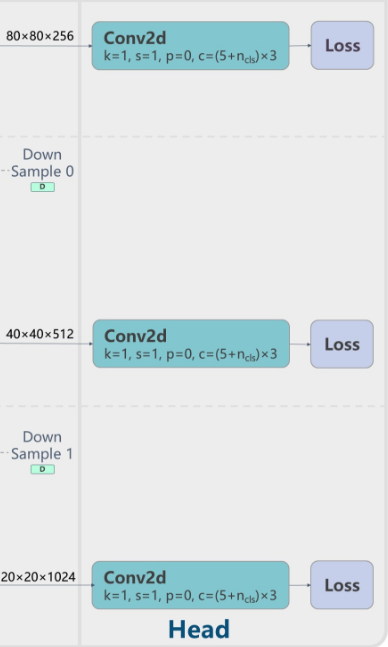
As shown in the figure above, YOLOv5 adopts a multi-scale detection mechanism, outputting feature maps at three different scales from the detection head to detect objects of various sizes. For a standard 640×640 input image, the shapes of the output tensors are:
- Large-scale feature map (P3 layer):
[batch_size, 3, 80, 80, 5+NC] - Medium-scale feature map (P4 layer):
[batch_size, 3, 40, 40, 5+NC] - Small-scale feature map (P5 layer):
[batch_size, 3, 20, 20, 5+NC]
The dimensions of each output tensor represent the following:
batch_size: The batch size, representing the number of images processed simultaneously.3: The number of anchor boxes predicted per grid cell; the default in the YOLOv5 model is 3.H, W: The height and width of the feature map (e.g., 80×80, 40×40, 20×20). With a 640x640 input, YOLOv5 outputs feature maps at 8x, 16x, and 32x downsampling scales, corresponding to resolutions of 80x80, 40x40, and 20x20, respectively.5+NC: The output dimensionality for each prediction box.
The information contained in the output of each prediction box is as follows:
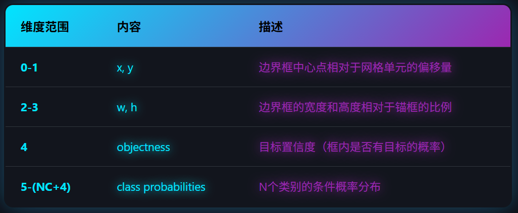
In summary, for the P3 layer output, a total of $80 \times 80 \times 3 = 19,200$ prediction boxes are generated; for the P4 layer output, $40 \times 40 \times 3 = 4,800$ prediction boxes; and for the P5 layer output, $20 \times 20 \times 3 = 1,200$ prediction boxes. Each prediction box contains (5+NC) lengths of information describing its attributes.
NMS Algorithm
As described above, when the YOLOv5 model performs inference on an image, it ultimately outputs over 20,000 prediction boxes across three scale dimensions, typically generating a large number of overlapping prediction boxes for the same object. Therefore, filtering is required to yield the final detection boxes. The process of filtering the model’s output tensor data to obtain these final detection boxes is known as the NMS algorithm. The task of the NMS algorithm is to select the most accurate box among overlapping ones, suppress (discard) other redundant boxes, and ultimately produce clear, non-overlapping detection results.
The basic execution workflow of the NMS algorithm is as follows:
- Sorting: Sort all prediction boxes output by the model in descending order based on their Confidence Score.
- Selection: Select the box with the highest confidence score and add it to the list of final output boxes.
- Suppression: Based on the highest-confidence prediction box selected in the previous step, calculate the Intersection over Union (IoU) between this box and all remaining boxes. Remove boxes whose IoU exceeds a preset threshold (e.g., 0.5), as they likely point to the same object.
- Loop: Repeat steps 2 and 3 until no boxes remain.
YOLOv5 introduces several improvements to the basic NMS algorithm:
- Unified processing of multi-scale prediction boxes: Since the inference output of the YOLOv5 model includes prediction boxes from three different feature maps (P3, P4, P5), all prediction boxes are concatenated together before NMS processing and then filtered uniformly. In this case, regardless of whether a prediction box comes from the P3 layer (responsible for small objects) or the P5 layer (responsible for large objects), as long as its confidence is high, it has the opportunity to be retained. The final selection is the highest-confidence box for that object.
- Support for multi-label and single-label detection: This option is controlled by the
multi_labelparameter. Whenmulti_label=False(single-label), each prediction box belongs to only a single class with the highest confidence, which is the most common object detection mode. Whenmulti_label=True(multi-label), a prediction box can belong to multiple classes simultaneously (e.g., an object is both a car and a taxi). In implementation, a single raw prediction box is split into multiple detection entries based on the number of classes exceeding the threshold. - Merge-NMS (Weighted Box Fusion): This is an optional post-processing step controlled by the
mergeparameter. Instead of discarding low-confidence boxes whose IoU exceeds the threshold, it calculates a weighted average between them and the high-confidence box. This theoretically improves localization accuracy by fusing positional information from multiple boxes.
Source Code Analysis of non_max_suppression
Below, we examine the execution logic and workflow of the NMS filtering algorithm applied to model outputs, referencing the non_max_suppression function in the YOLOv5 source code.
The
non_max_suppressionfunction in the YOLOv5 source code is located inutils/general.py.
The prediction data obtained from the YOLOv5 model by the non_max_suppression function is a tensor of shape [batch_size, num_boxes, 5 + nc]. Here, batch_size is the number of images fed into the model for inference in a single batch, num_boxes corresponds to the total number of prediction boxes per image inference (25,200 = 19,200 + 4,800 + 1,200), and 5 + nc represents the predicted output data for each box (center_x, center_y, width, height, object_confidence, class_1, …, class_n).
The key procedural code snippets of the non_max_suppression implementation are excerpted and explained below:
# NMS algorithm implementation
def non_max_suppression(
    prediction,
    conf_thres=0.25,
    iou_thres=0.45,
    classes=None,
    agnostic=False,
    multi_label=False,
    labels=(),
    max_det=300,
    nm=0,  # number of masks
):
The above is the declaration of the non_max_suppression function in the YOLOv5 source code, where:
prediction: The raw prediction data output by the model, containing information for all detection boxes across the small, medium, and large scales.conf_thres: The confidence threshold used to control and filter low-confidence detection boxes during NMS. A detection box is retained for subsequent processing only when its confidence (including object confidence and class confidence) is greater than this threshold. Increasing this value reduces the number of detection boxes but may miss some true objects; lowering it increases the number of boxes but may introduce more false positives. This value is set based on precision and recall requirements.iou_thres: The IoU (Intersection over Union) threshold used in the NMS algorithm to determine if bounding boxes overlap. When the IoU between two detection boxes exceeds this threshold, NMS keeps the one with higher confidence and removes the lower-confidence one. Increasing this value retains more overlapping detection boxes; lowering it removes overlapping boxes more aggressively.classes: Specifies that only detection results of particular classes should be retained. If set to a list of class indices, the function returns only detection boxes for those classes, filtering out others.agnostic: Controls whether class-agnostic NMS processing is performed.- When
False(default), NMS is performed independently within each class, and overlapping boxes of different classes do not suppress each other. - When
True, NMS treats all classes as a single class, and overlapping boxes suppress each other regardless of their class.
- When
multi_label: Controls whether multi-label detection is allowed (i.e., an object may belong to multiple classes, such as a detection result being both a person and a man).- When set to
False(default), each detection box retains only the single class with the highest confidence. - When set to
True, a detection box can retain all classes whose confidence exceeds theconf_thresthreshold.
- When set to
labels: Used in auto-labeling mode to pass prior label information.max_det: Limits the maximum number of detection boxes output per image. By default, a maximum of 300 valid detection boxes are output per image.nm: Specifies the number of masks, used only for segmentation models.
bs = prediction.shape[0]  # batch size
    nc = prediction.shape[2] - nm - 5  # number of classes
    xc = prediction[..., 4] > conf_thres  # candidates: boxes with confidence > threshold are true, otherwise false
The batch size bs is read from the prediction tensor. The model can predict multiple images at once, and the first dimension of its prediction tensor is the number of images bs. nc is the number of classes output by the model, where nm is only used for segmentation models and is 0 for standard object detection models. xc compares the object confidence of all detection boxes in the prediction output against the confidence threshold conf_thres. Boxes with a confidence greater than the threshold are marked as true, and others as false. In fact, the vast majority of prediction boxes output by prediction are filtered out at this confidence threshold comparison step.
output = [torch.zeros((0, 6 + nm), device=prediction.device)] * bs
    # Iterate over the inference results for each image
    for xi, x in enumerate(prediction):  # image index, image inference
An output variable is declared to store the valid detection boxes after subsequent NMS filtering, where the detection information length for each box is 6 (coordinate positions + confidence + class). A for loop then extracts each image frame from the prediction variable for independent processing, and all subsequent operations within this loop target a single image frame.
x = x[xc[xi]]  # confidence: retain only detection boxes with confidence > conf_thres

        # If none remain process next image
        if not x.shape[0]:  # If the current image has no detection boxes, skip and process the next image
            continue
Using x = x[xc[xi]], x retains only the detection boxes of the xi-th image whose confidence is greater than conf_thres, discarding all other boxes. It then checks whether the number of detection boxes in the x list is 0. If it is 0, it means no valid targets were detected in the current image frame, and the loop directly continues to process the next image frame.
At this point, the x list holds all detection box information with a confidence $> \text{conf_thres}$ detected in the current image frame.
# Compute conf: Multiply each detection box's confidence by its class confidence to get the final confidence for each class per box
        x[:, 5:] *= x[:, 4:5]  # conf = obj_conf * cls_conf

        # Box/Mask
        box = xywh2xyxy(x[:, :4])  # convert (center_x, center_y, width, height) to (x1, y1, x2, y2)
The information of all detection boxes in the x list is processed: the classification probability for every class is multiplied by the overall object confidence to obtain the absolute probability for each class; the xywh coordinate information output by the model is converted into the xyxy format required by the NMS algorithm.
# Format the detection matrix x, which contains prediction box coordinates, confidence, and class confidences
        if multi_label: # For multi-label, retain all classes in the cls section whose confidence exceeds the threshold
            i, j = (x[:, 5:mi] > conf_thres).nonzero(as_tuple=False).T
            x = torch.cat((box[i], x[i, 5 + j, None], j[:, None].float(), mask[i]), 1)
        else:  # best class only: for single label, retain only the class with the highest confidence that exceeds the threshold
            conf, j = x[:, 5:mi].max(1, keepdim=True)
            x = torch.cat((box, conf, j.float(), mask), 1)[conf.view(-1) > conf_thres]
The code above formats the detection box list needed by the NMS algorithm and performs a preliminary round of filtering using the absolute class probabilities. It is divided into multi-label and single-label cases:
- In the multi-label case, the absolute probability of each class is compared with the confidence threshold
conf_thres, and all classes with absolute probabilities greater than the threshold are retained. - In the single-label case, the class with the highest absolute probability is found among all classes and compared against the confidence threshold
conf_thres. If it exceeds the threshold, it is retained.
At this point, each detection box in the x list contains only a single class, formatted as [x1, y1, x2, y2, confidence, class]. If a detection box supports two classes simultaneously (when multi_label is enabled), there will be two separate detection boxes for it in the x list.
# Filter by class
        if classes is not None: # Retain only classes specified by the classes parameter, ignore others
            x = x[(x[:, 5:6] == torch.tensor(classes, device=x.device)).any(1)]

        # Check shape
        n = x.shape[0]  # number of boxes
        if not n:  # no boxes
            continue
If the classes parameter is set, only the categories specified by classes are retained in the x list, and all other detection box information is filtered out. The code then checks the number of remaining detection boxes. If it equals 0, it proceeds directly to process the next image frame.
# Sort prediction boxes based on confidence and retain only the top max_nms prediction boxes
        x = x[x[:, 4].argsort(descending=True)[:max_nms]]  # sort by confidence and remove excess boxes

        # Batched NMS
        # Determine whether subsequent NMS filtering needs to distinguish between different classes based on the agnostic parameter
        c = x[:, 5:6] * (0 if agnostic else max_wh)  # classes
        boxes, scores = x[:, :4] + c, x[:, 4]  # boxes (offset by class), scores

        # The result of nms is an index array containing the indices of prediction boxes retained by the NMS algorithm
        i = torchvision.ops.nms(boxes, scores, iou_thres)  # NMS: Call torchvision's NMS function
This section reaches the core processing steps of the NMS algorithm. First, all detection boxes in the x list are sorted in descending order of confidence, and only the top max_nms prediction boxes are retained. Then, based on the setting of the agnostic parameter, it decides whether subsequent NMS filtering should distinguish between different classes. When agnostic=False, the class index is multiplied by a large number max_wh (default is 7680), ensuring that different classes are computed in separate spatial regions so they do not suppress each other during NMS filtering.
Finally, the coordinates boxes and detection confidence scores of each detection box are extracted from the x list, and torchvision.ops.nms is called to perform NMS filtering. torchvision.ops.nms returns a 1D integer tensor containing the indices of the bounding boxes that should be retained after the NMS algorithm, ordered by confidence from highest to lowest.
i = i[:max_det]  # limit detections: retain at most the top max_det NMS outputs
        if merge and (1 < n < 3e3):  # Merge NMS (boxes merged using weighted mean)
            # update boxes as boxes(i,4) = weights(i,n) * boxes(n,4)
            iou = box_iou(boxes[i], boxes) > iou_thres  # iou matrix
            weights = iou * scores[None]  # box weights
            x[i, :4] = torch.mm(weights, x[:, :4]).float() / weights.sum(1, keepdim=True)  # merged boxes
            if redundant:
                i = i[iou.sum(1) > 1]  # require redundancy

        output[xi] = x[i]
The code above restricts the return result of torchvision.ops.nms to a maximum of the first max_det results as the final output. When the merge feature is enabled, IoU comparisons are used to fine-tune the coordinate positions of the final output detection boxes, enhancing localization accuracy.
The final step assigns the NMS-filtered detection box list to output as the final output of the non_max_suppression function.