Detailed Explanation of P, R, PR, and F1 Metrics for Computer Vision Object Detection Models

The four image files F1_curve, P_curve, PR_curve, and R_curve generated in the YOLOv5 model training results correspond to the F1, P, PR, and R metric curves after model training completion, respectively. This article provides a detailed summary and organization of these four metrics.

P_Curve

The P curve corresponds to the model’s Precision, which measures out of all samples predicted by the model as positive, how many are actually true positives. It focuses on the accuracy of the prediction results, answering the question: “How accurate are the detections?” The higher the precision, the fewer false positives and misjudgments (mistaking the background or other objects as the target) the model makes. For example, in security surveillance, high precision means high alarm accuracy, reducing false alarms. The figure below shows a typical P_Curve:

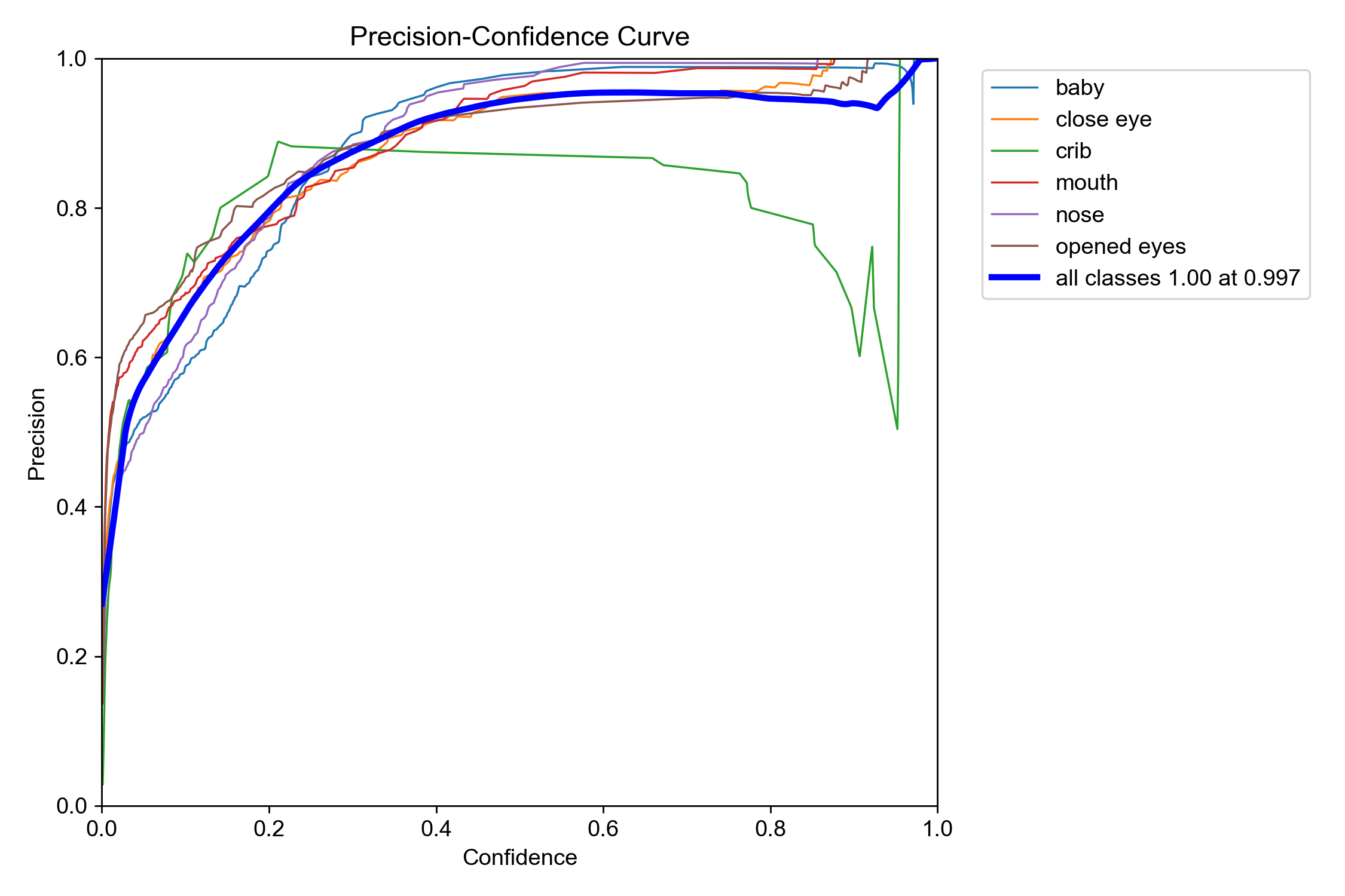
As can be seen, the vertical axis of the P_Curve is Precision, and the horizontal axis is Confidence. As the confidence threshold increases, precision generally shows an upward trend. This is easy to understand: the lower the confidence, the more misjudged targets are counted in, which naturally pulls down the precision metric. As the confidence threshold increases, a large number of low-confidence detection results are filtered out, misjudgments decrease, and the precision metric naturally rises.

In an ideal scenario, the P_Curve is a straight line where Precision remains consistently around 1.0. This means that no matter how you set the confidence threshold, the model’s predictions are extremely reliable with very few false detections. Of course, this situation is impossible in reality. In most cases, the P_Curve presents a curve where Precision rapidly rises as the Confidence threshold increases, until a certain point where the vertical axis coordinate approaches 1 and remains flat thereafter. However, the larger the area enclosed under the P_Curve (which actually means Precision can approach 1 more quickly), the higher the model’s robustness, indicating that it can maintain high precision across different thresholds.

If only a few class curves (such as the crib curve in the above image) are significantly lower than the others, it may indicate that the number of samples for that class in the dataset is insufficient (which is often the case) or that the sample quality is poor, making it difficult for the model to accurately learn the features of that class. In this case, you should consider collecting more data or performing data augmentation for that category. Additionally, under normal circumstances, the P_Curve should rise smoothly. If the curve exhibits drastic fluctuations or abnormal sharp drops, it may suggest overfitting or underfitting problems during the training process, requiring targeted treatment.

The primary value of the P_Curve lies in assisting with the scientific configuration of the confidence threshold for model predictions, achieving a balance between Precision and Recall to meet project application requirements and goals. For example, in application scenarios where false detections are unacceptable and high precision is pursued (such as high costs for false alarms in security monitoring), a confidence threshold corresponding to high precision (such as 0.95 or higher) should be selected based on the P_Curve. In this case, the model’s output will be very conservative, outputting only results it is extremely certain of, at the cost of potentially missing some less certain positive samples, thereby leading to a lower recall.

R_Curve

Corresponding to the P curve is the R curve, which is the Recall curve. Recall measures out of all true positive samples, how many were successfully predicted by the model. Therefore, the Recall metric focuses on the model’s ability to discover positive examples, answering the question: “How complete are the detections?” The higher the recall, the fewer false negatives (failing to detect a true target) the model produces.

Similar to the P curve, the horizontal axis of the R curve is also Confidence, and the vertical axis is the model’s Recall. Thus, it illustrates how recall changes when the confidence threshold of the model’s output varies from 0 to 1. The figure below shows a typical recall curve:

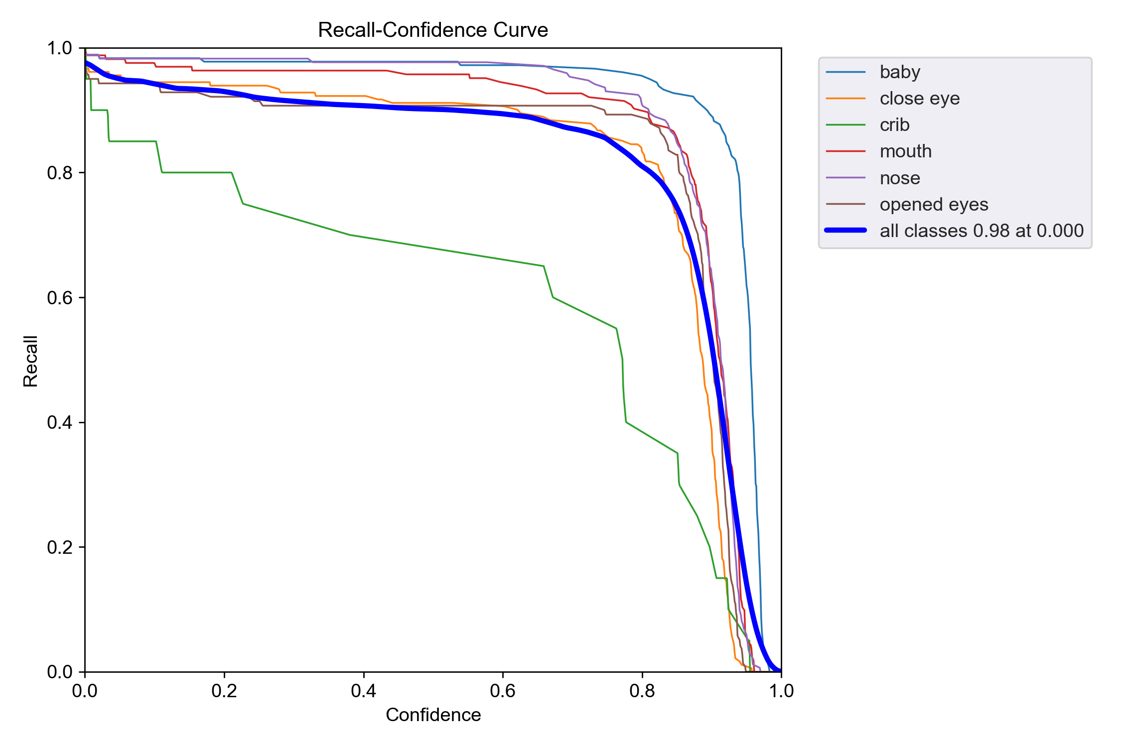
Both the P_Curve and R_Curve use the confidence threshold (Confidence) as the horizontal axis, but the changes in these two metrics relative to the confidence threshold are exactly opposite. In the R_Curve, as the confidence threshold increases, the recall exhibits a downward trend. This is also relatively intuitive to understand: higher confidence leads to more positive case judgments being filtered out (because the confidence does not meet the threshold requirement), which naturally leads to increased missed detections and lower recall.

The higher the overall position of the R_Curve in the above image, and the larger the area enclosed by the curve and the two coordinate axes, the more robust the model’s performance and the fewer missed detections it has, as it maintains high recall across different confidence thresholds.

Similarly, the primary value of the R curve is to help scientifically select and set the confidence threshold to balance Precision (P) and Recall (R) while meeting application requirements. For example, in application scenarios that pursue high recall and completely unacceptable missed detections (such as medical diagnosis, obstacle detection in autonomous driving, etc.), a confidence threshold corresponding to an acceptable high recall (such as 0.95 or higher) should be selected based on the R curve.

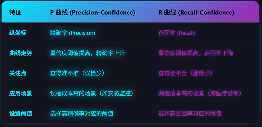
The figure below is a comparison and summary table of the P curve and the R curve:

PR Curve

The PR Curve (Precision-Recall Curve) is a core tool for evaluating the performance of object detection models. It intuitively displays the trade-off relationship between Precision and Recall under different confidence thresholds.

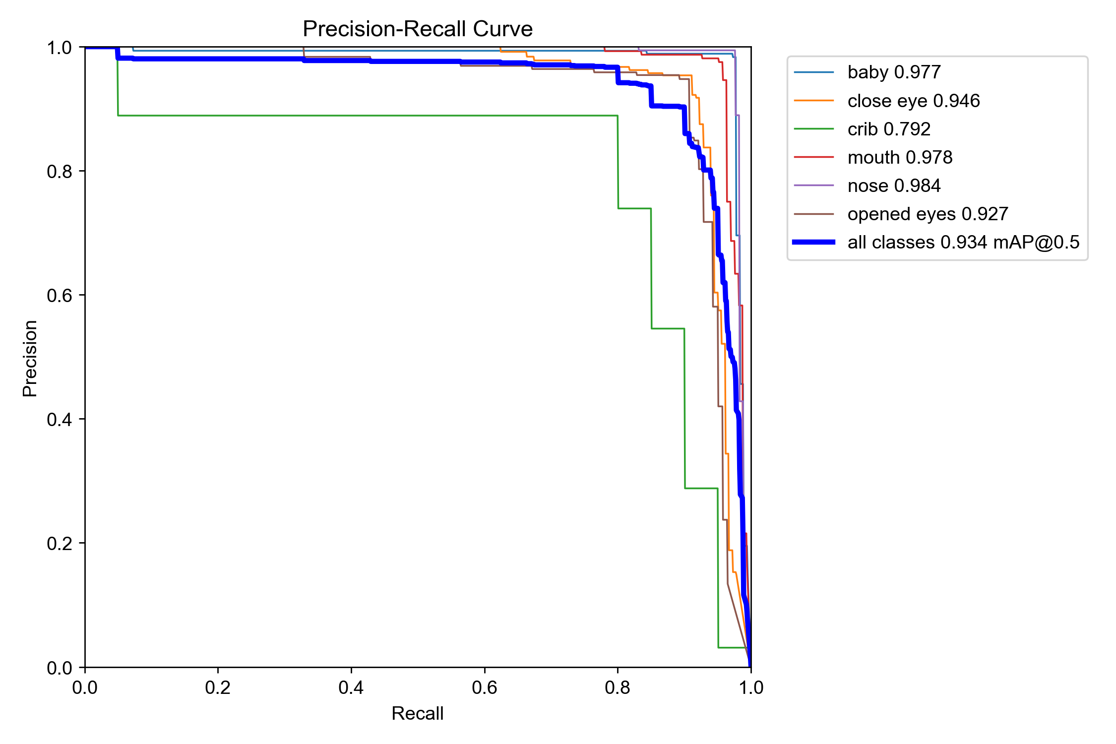
The PR curve uses Recall as the horizontal axis and Precision as the vertical axis. Each point on the curve represents the combination of precision and recall achieved by the model at a specific confidence threshold. The figure below is an example of a typical PR curve:

The plotting process for the PR curve of a specific category is as follows:

• First, sort all predicted bounding boxes generated by the model on the validation set in descending order of their confidence scores.
• Then, iterate through thresholds, starting from the highest confidence (e.g., 0.99) and gradually lowering the threshold (e.g., 0.98, 0.97, …, 0.01). At each threshold, treat all prediction boxes with a confidence higher than that threshold as positive examples, and calculate the precision and recall at this point.
• Finally, connect all calculated (Recall, Precision) points to form the PR curve.

Typically, the shape of the PR curve is a curve that starts from the top-left corner and gradually descends towards the bottom-right corner. This means that as recall increases (wanting to detect more true targets), precision will gradually decrease (false detections will increase). Conversely, if you want to increase precision (reduce false detections), recall will decrease (missed detections will increase).

When comparing the performance of two models (using different models tested on the same validation dataset, of course), if model A’s PR curve completely encloses model B’s PR curve, it can be asserted that model A’s performance is superior to model B’s. If the two curves intersect, it is necessary to compare their pros and cons by calculating the area between each curve and the two axes (which is essentially the AP metric).

Relationship Between PR Curve and AP/mAP Metrics

While the PR curve is intuitive, it is not a single specific number, making it inconvenient to use—especially when comparing different models. Therefore, the AP and mAP metrics were introduced based on the PR curve.

The AP (Average Precision) metric refers to the area between the PR curve and the two coordinate axes. A higher AP value indicates that the model can maintain high precision while maintaining high recall, resulting in better comprehensive performance. Of course, the AP metric is specific to a single detection category.

Since most object detection models support detecting targets of multiple different categories, comparing the overall performance of models requires evaluating the average AP metric across all target categories. This average AP metric is the mAP (mean Average Precision) metric. The mAP metric is the average of the AP values for all categories supported by the object detection model after training, and it is currently the most authoritative and commonly used evaluation metric in the field of object detection.

F1 Curve

Once you fully understand the P and R curves discussed above, the F1 curve becomes quite easy to grasp. The F1 score is the harmonic mean of Precision and Recall, used to comprehensively evaluate model performance. Its calculation formula is:

$$ F1 = 2 * (Precision * Recall) / (Precision + Recall) $$

Since both Precision and Recall metrics are decimals between 0 and 1, the F1 score calculated by the above formula also ranges between 0 and 1. A higher F1 score indicates better comprehensive performance of the model in terms of precision and recall. The figure below shows a typical F1 curve:

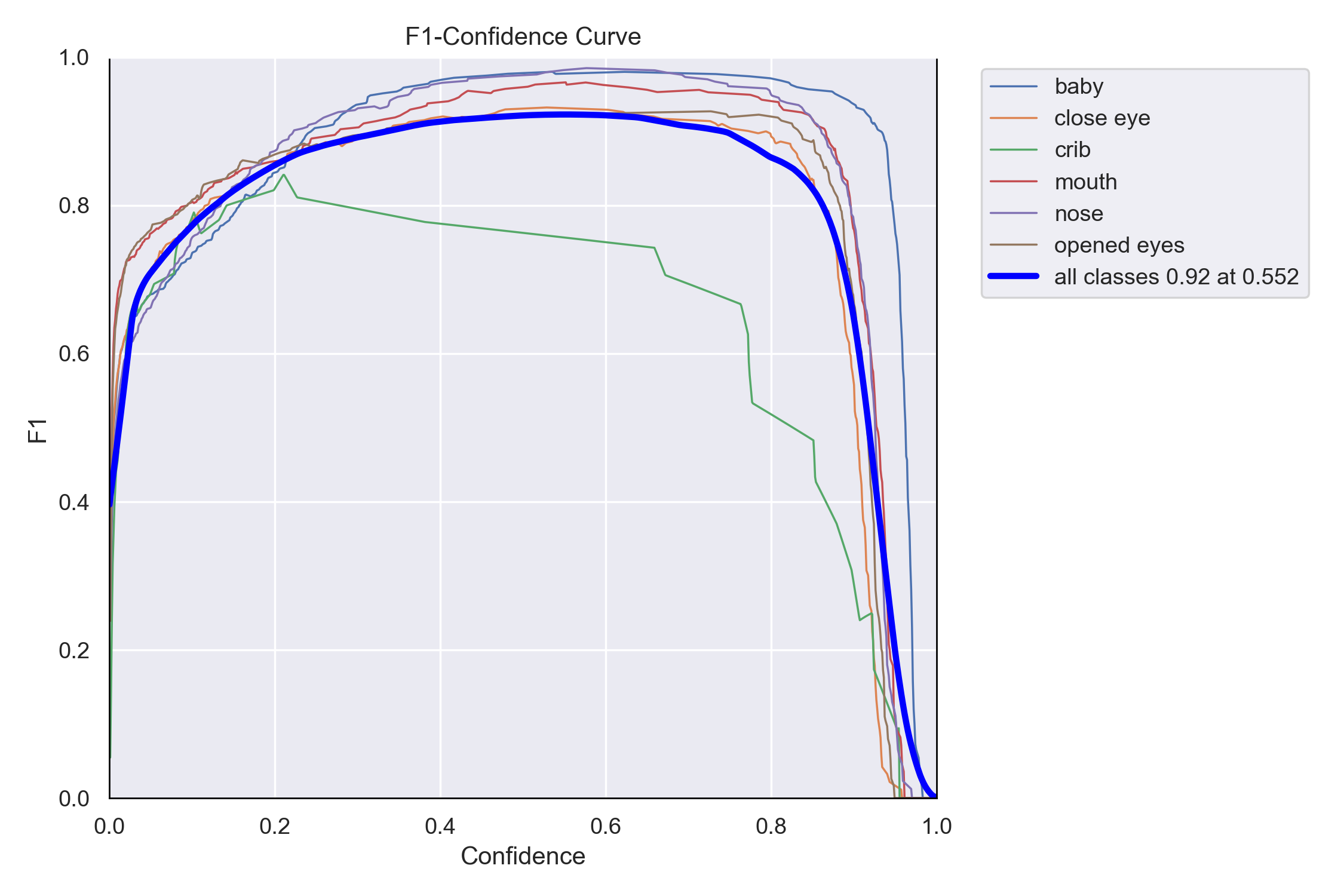
As can be seen from the above figure, the F1 curve also uses the confidence threshold (Confidence) as its horizontal axis, and the vertical axis represents the F1 score under different confidence levels. Under normal circumstances, the F1 curve typically presents a bell shape that first rises and then falls. At lower confidence thresholds, the model predicts many results (high recall $R$), but they contain a large number of false detections (low precision $P$), resulting in a lower F1 score at low confidence levels. As the threshold increases, false detections decrease, precision rises, and the F1 score rises accordingly. After reaching a peak, continuing to increase the threshold filters out some correct predictions (low recall), thereby causing the F1 score to drop.

• High and wide curve shape: If the sides of the F1 curve are steep and form a wide plateau at a higher position, it indicates that the model can maintain high performance over a wide range of confidence thresholds, making the model very robust. This is the ideal shape for an F1 curve.
• Low and narrow curve shape: If the overall position of the F1 curve is low and the peak is sharp, it means that the model performs moderately well only under very specific thresholds, and its overall generalization ability is poor.

Overall, the F1 curve is closely related to the P curve (Precision-Confidence) and R curve (Recall-Confidence), and together they form a complete evaluation system. Combining all three can assist in a more scientific selection of the optimal confidence threshold for model inference based on specific application requirements:

• In application scenarios that pursue high precision (avoiding false detections), you can choose a higher threshold to the right of the peak point, sacrificing some recall in exchange for higher precision.
• In application scenarios that pursue high recall (avoiding missed detections), you can choose a lower threshold to the left of the peak point, sacrificing some precision in exchange for higher recall.