An Interpretation of the YOLOv5 Model Network Architecture

26 Oct, 2025
- AI

Based on the P3 version of YOLOv5, this article provides a detailed summary of its overall network architecture and the working logic of each sub-module, laying a solid foundation for further in-depth study of the YOLOv5 model.

Note: The YOLOv5 version summarized in this article is YOLOv5l, v6.0, P5 version. For details on the differences between various versions, please refer to Summary of Different Versions of the YOLOv5 Model.

Backbone Network

Before presenting a complete summary of the entire backbone network structure, the individual sub-modules within the backbone are organized into subsections below.

Focus and 6x6 Convolution

Early versions of YOLOv5 utilized a Focus structure (a slicing operation) at the beginning of the backbone network to reduce computational load while preserving information. This module is primarily used for image downsampling and feature extraction. By reducing spatial resolution while retaining more original information, the essence of this operation is to convert spatial information (width and height) into the channel dimension.

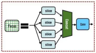
The operation of the Focus module consists of three steps:

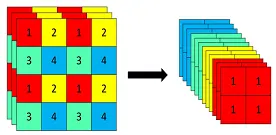
Slicing operation: Samples the input image every other pixel along the width and height directions to obtain 4 complementary sub-feature maps.
Channel concatenation: Concatenates the 4 sub-feature maps along the channel dimension, which effectively quadruples the number of channels.
Convolution operation: Applies a standard convolution to the concatenated feature map.

Taking the structure of YOLOv5s as an example, an original 608x608x3 image is input into the Focus module. After the slicing operation, it becomes a 304x304x12 feature map, and then through a 1x1 convolution operation with 32 filters, it outputs a 304x304x32 feature map.

The processing of the slicing operation is shown in the figure below: As can be seen, this Slice operation is completely identical to the Reorg operation in the YOLOv2 model (refer to Interpretation of the YOLOv2 Model Network Architecture).

The workflow of Focus processing is illustrated in the figure below:

However, in later versions of YOLOv5 (such as after v6.0), the Focus structure was replaced by a standard convolutional layer with a kernel size of 6 and a stride of 2 (Conv2d 6x6, stride=2). This is why some architectural diagrams of different YOLOv5 versions show the Focus module while others show the 6x6 convolution module. Although the Focus module theoretically reduces information loss, in practical applications, a well-designed convolutional layer (using a larger 6x6 kernel) can also effectively capture similar spatial information. Moreover, on hardware such as GPUs, standard convolutions are usually highly optimized, and actual inference speeds may turn out to be advantageous or comparable. Therefore, in newer versions of YOLOv5, replacing the special Focus structure with a general convolutional layer makes the overall network structure more unified and concise, reduces custom modules, and lowers code complexity and maintenance costs.

Activation Function

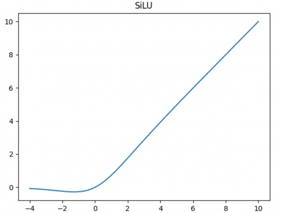
In the backbone network of YOLOv5, the SiLU activation function (also known as the Swish function) is universally used to replace the LeakyReLU commonly used in previous versions. Compared to LeakyReLU, the SiLU activation function is smoother around zero, which helps improve gradient flow and the expressive power of the model.

The formula for the SiLU activation function is:

$$ f(x)=x * Sigmoid(x) $$

Where $Sigmoid(x)$ is the standard sigmoid function, with values ranging between 0 and 1. The characteristics of the SiLU function are non-linearity and continuous differentiability.

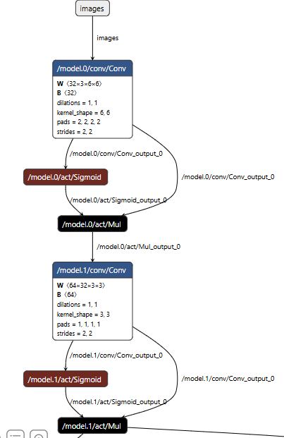
The figure below shows the structure of the first two convolutional blocks of the backbone network’s image input, viewed via Netron from the YOLOv5 ONNX file. The calculation process of the SiLU activation function is clearly visible in this structural diagram, which can be decomposed into two distinct steps:

Sigmoid transformation: First, the output of the convolutional layer is fed into the Sigmoid function. The Sigmoid function maps the value of each element into the interval $(0, 1)$.
Element-wise multiplication: Next, the original input is multiplied element-wise with the Sigmoid weights obtained in the first step. This step corresponds to the act/Mul operation in the figure below. Its effect is to amplify (weight close to 1), suppress (weight close to 0), or partially retain (weight between 0 and 1) the original features based on the weights calculated by Sigmoid.

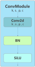
However, it should still be noted that different versions of YOLOv5 use different activation functions. Their early versions (such as v1.0-v3.0) still defaulted to LeakyReLU, which is why a large number of CBL (Conv-BN-LeakyReLU) blocks can still be found in the backbones of these early versions. Starting around version v5.0, the official implementation completely switched the default activation function to SiLU, and the CBL blocks consequently became Conv-BN-SiLU. This is the reason why most YOLOv5 model architecture diagrams found online still heavily employ CBL blocks and LeakyReLU activation functions.

CSPLayer

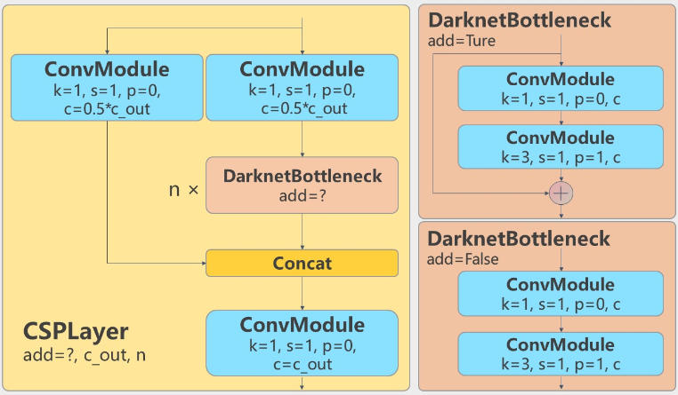
Similar to YOLOv4, YOLOv5 also adopts the CSP (Cross Stage Partial) structure in the implementation of its backbone network. In other words, the feature map is split into two parts along the channel dimension; one part undergoes complex convolutional transformations, while the other part takes a shortcut, and finally, the two parts are merged before output. Conceptually, there is no significant difference from YOLOv4. For a more detailed explanation of CSP processing, please refer to Interpretation of the YOLOv4 Model Network Architecture.

The structure of the CSP blocks in YOLOv5 is shown in the figure below. As can be seen, there are two types of CSP blocks used in the YOLOv5 model structure:

CSP1 is used in the backbone network, where the convolutional transformation part utilizes ResNet’s residual block structure (such as the DarknetBottleneck add=true part in the figure below).
CSP2 is used in the neck network, where the convolutional processing part consists simply of two consecutive convolutional blocks (such as the DarknetBottleneck add=false part in the figure below).

SPPFBottleneck

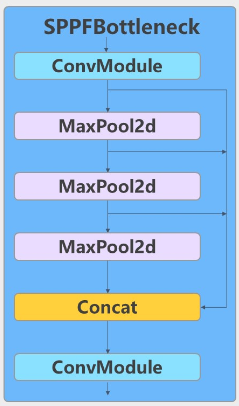
The full name of the SPPF module is Spatial Pyramid Pooling-Fast. It is essentially still an SPP module, but optimized for computational speed and performance.

The core objective of both SPPF and SPP modules is to expand the receptive field of feature information and fuse multi-scale context information. The difference between the two is simply that the traditional SPP module processes the input feature map in parallel using multiple large pooling kernels (such as 5x5, 9x9, 13x13) and concatenates the results, whereas the SPPF module applies the same 5x5 pooling kernel repeatedly in a cascading manner multiple times, and then concatenates the pooling results from different stages.

Regarding the working logic of the SPP module, you can refer to another note: Interpretation of the YOLOv4 Model Network Architecture.

Compared to the former, the cascading approach of the SPPF module using identical pooling kernels is easier to optimize on hardware, yields faster computation speeds, and can effectively enhance the model’s adaptability to objects of different scales. It achieves faster inference speeds while maintaining or even improving model performance.

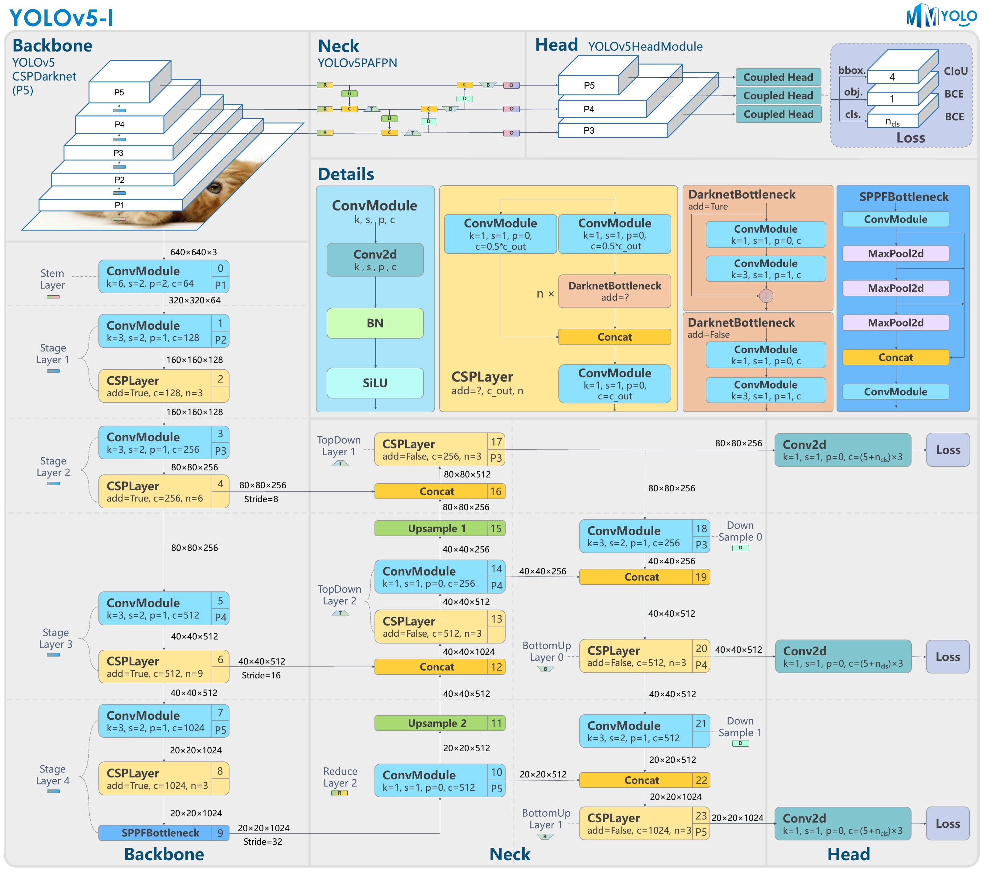
At this point, the backbone network of the YOLOv5 model becomes clear: assuming an input image resolution of 640x640, the backbone network outputs three sets of feature information with different resolutions and channel counts at scaling factors of 8x, 16x, and 32x respectively, which are then passed to the neck network for feature detection.

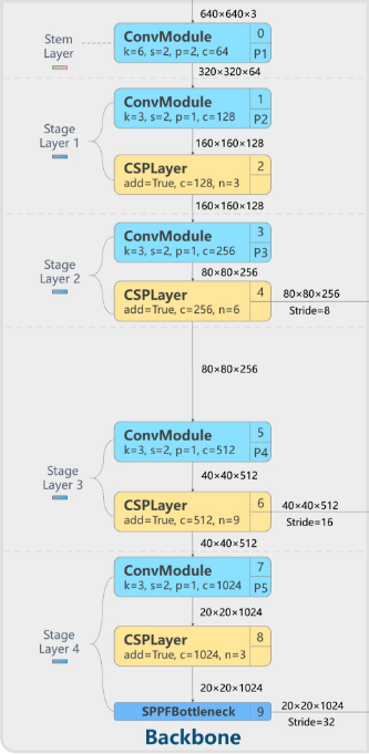
In summary, the entire backbone network can be divided into five parts from top to bottom:

Stem Layer: This is the Focus module introduced above, although in newer model versions, the Focus module has been replaced by a standard convolutional network with a 6x6 kernel and a stride of 2. With an input image resolution of 640x640x3, this module outputs a feature map of dimensions 320x320x64.
From Layer 1 to Layer 3, the structure consists of a 3x3 convolution followed by multiple consecutive CSP blocks. The preceding 3x3 convolutional module with a stride of 2 is responsible for halving the resolution of the input feature map while doubling the number of channels.
- Layer 1 contains 1 3x3 convolution + 3 consecutive CSP blocks, outputting a feature map of dimensions 160x160x128.
- Layer 2 contains 1 3x3 convolution + 6 consecutive CSP blocks, outputting a feature map of dimensions 80x80x256. The output of this layer is fed into the neck network as the large-resolution feature map.
- Layer 3 contains 1 3x3 convolution + 9 consecutive CSP blocks, outputting a feature map of dimensions 40x40x512. The output of this layer is fed into the neck network as the medium-resolution feature map.
For the final Layer 4, the first half of the processing remains identical to Layers 1–3, containing 1 3x3 convolution + 3 consecutive CSP blocks, with the addition of an extra SPPFBottleneck module at the end to further expand the receptive field of the output feature map. The output of this layer is a feature map of dimensions 20x20x1024. Finally, this layer’s output is fed into the neck network as the small-resolution feature map.

Neck Network

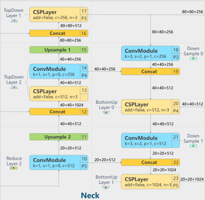
The neck network is a core component for YOLOv5 to achieve multi-scale object detection. Its objective is to efficiently fuse the features extracted by the backbone network, enabling the model to simultaneously recognize objects of varying sizes.

Overall, the architecture and concepts of YOLOv5 and YOLOv4’s neck network designs have not changed drastically. However, the core difference is that YOLOv5 introduces improvements such as the CSP2 module (described in the backbone section above) into its neck network, which significantly strengthens feature fusion capabilities and enhances computational efficiency.

Regarding the overall network architecture, the neck network of YOLOv5 still adopts the dual-directional structure of FPN (Feature Pyramid Network) + PAN (Path Aggregation Network) shared with YOLOv4. Here, the FPN is responsible for passing strong semantic features top-down, while the PAN is responsible for passing accurate localization features bottom-up, forming a powerful feature pyramid.

FPN processing: Through a Concat operation along the channel dimension, the upsampled deep feature maps are concatenated with the corresponding shallow feature maps, combining the detail information from shallow layers with the semantic information from deep layers.
PAN processing: In the PAN path, convolutional layers with a stride of 2 are used to downsample the fused feature maps once again for further fusion with higher-level features.

Head

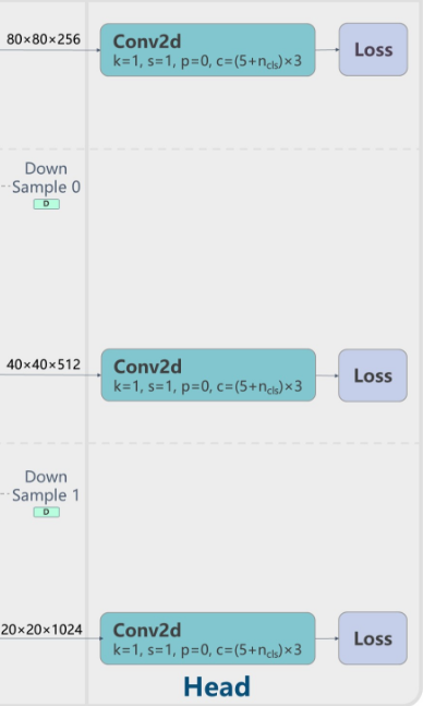
Compared to previous versions, the detection head does not show significant differences. The three paths of output feature maps undergo independent 1x1 convolution processing to output detection result tensors of various resolutions.

Overall Network Architecture of the YOLOv5 Model

Finally, here is the overall network architecture diagram of the YOLOv5 model. Combined with the descriptions of each sub-module above, understanding the overall architecture diagram becomes much easier: