Summary of YOLOv3 Evolution: Output, Anchors, and Loss Functions
- 19 Oct, 2025
This article summarizes the YOLOv3 model, focusing on the organization format of output data, anchor prediction boxes, and the calculation of loss functions.
The Output of the YOLOv3 Model
As shown in the overall architecture diagram of the YOLOv3 model below, unlike earlier YOLOv1 and YOLOv2 models which output only a single set of 3D tensors and learn/interpret object positions and categories from it, the YOLOv3 model ultimately outputs three independent sets of 3D tensors. These are used to locate and detect objects of different sizes, respectively.
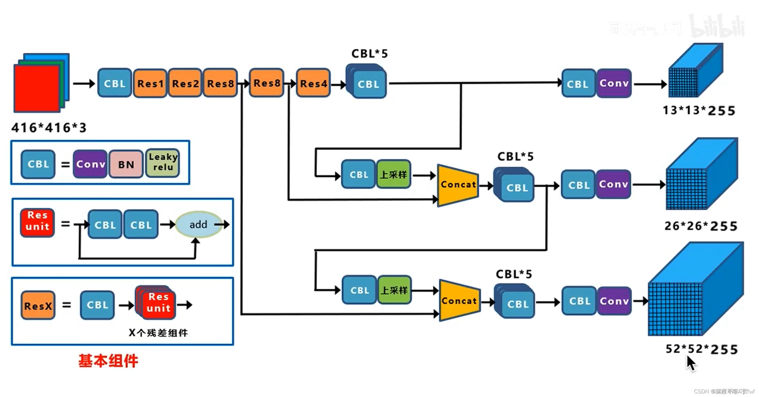
Taking the 13x13x255 3D tensor output in the figure above as an example, the input image is divided into a 13x13 grid. Each grid presets three anchor prediction boxes with different sizes and aspect ratios (for information regarding YOLOv3 anchor boxes, refer to the next section). Then, a 1D vector of length 255 is used to describe the object information detected in that grid (where the center of the object falls within that grid). In other words, this vector of length 255 contains information for 3 prediction boxes, as illustrated below.
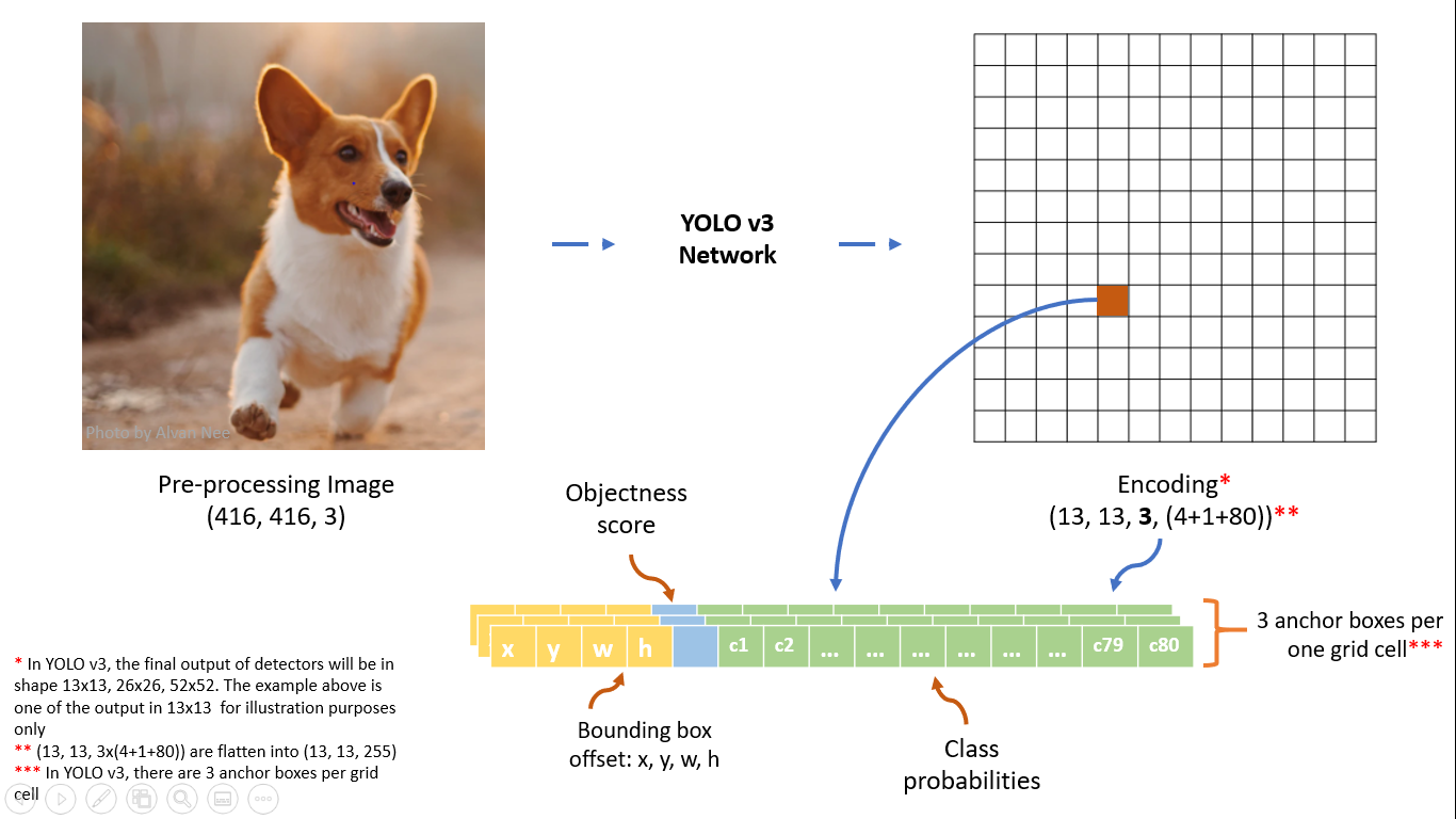
The information contained in each prediction box is identical to the output of a single prediction box in YOLOv2: center coordinate positions + width and height + prediction confidence + recognition information for 80 classes (for the COCO dataset). Thus, the information length for each prediction box is 4 + 1 + 80 = 85, and the information length for the 3 prediction boxes contained in a single grid is 255. This is the explanation and origin of the dimensions for the 13x13x255 3D tensor.
If each grid places $B$ anchor boxes and the model supports $C$ object classes to be detected, the output data length per grid will be $B \times (4 + 1 + C)$.
YOLOv3 Anchor Boxes
Regarding the design of anchor boxes within the grid, YOLOv3 continues to adopt the prior anchor boxes introduced in the YOLOv2 model. However, while YOLOv2 places 5 anchor boxes in advance per grid, YOLOv3 places 3 anchor boxes per grid (as explained in the tensor output section above).
As for the size selection of the anchor priors, YOLOv3 follows the same approach as YOLOv2, using the k-means clustering method on the training dataset to derive the sizes of 9 prior boxes matching that dataset.
- For details on how to use the k-means clustering method to obtain dataset anchor priors, please refer to the article Detailed Explanation of the Anchor Mechanism in YOLOv2, which provides a very detailed description of the calculation pipeline for deriving anchor box aspect ratios from a dataset.
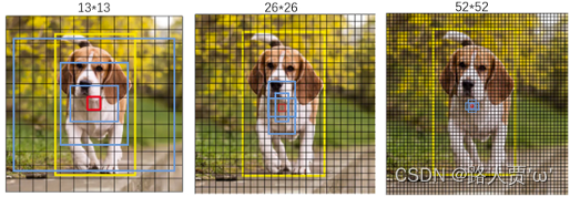
In the YOLOv3 paper, the authors calculated the sizes of 9 anchor priors based on the COCO dataset. Sorted by area size and divided evenly into 3 parts, they target feature maps of different resolutions:
- 3 large boxes, targeting 13×13 resolution feature maps (totaling 13x13x3 = 507 prediction boxes), responsible for large object detection: (116×90), (156×198), (373×326)
- 3 medium boxes, targeting 26×26 resolution feature maps (totaling 19x19x3 = 2028 prediction boxes), responsible for medium object detection: (30×61), (62×45), (59×119)
- 3 small boxes, targeting 52×52 resolution feature maps (totaling 52x52x3 = 8112 prediction boxes), responsible for small object detection: (10×13), (16×30), (33×23)
YOLOv3 Loss Function Optimization
As summarized above, the YOLOv3 model outputs three independent sets of 3D tensors to detect objects of varying sizes. Consequently, its loss function must be applied independently to each of these three outputs. The loss functions used to calculate loss values for the three outputs are completely identical, and their calculation processes run entirely independently without mutual interference. This yields three loss values: Loss_13, Loss_26, and Loss_52. The total loss of the entire model is simply the sum of these three loss values.
Regardless of which scale is being evaluated, the YOLOv3 loss function consists of the following three components:
- Bounding Box Regression Loss (
lbox): Responsible for evaluating the accuracy of the prediction box position (center coordinates $x, y$) and size (width and height $w, h$). - Confidence Loss (
lobj): Responsible for determining whether a target object is contained within the prediction box. - Classification Loss (
lcls): Responsible for determining the specific class of the object within the prediction box.
Therefore, the calculation pipeline for the overall model loss function is illustrated in the diagram below:
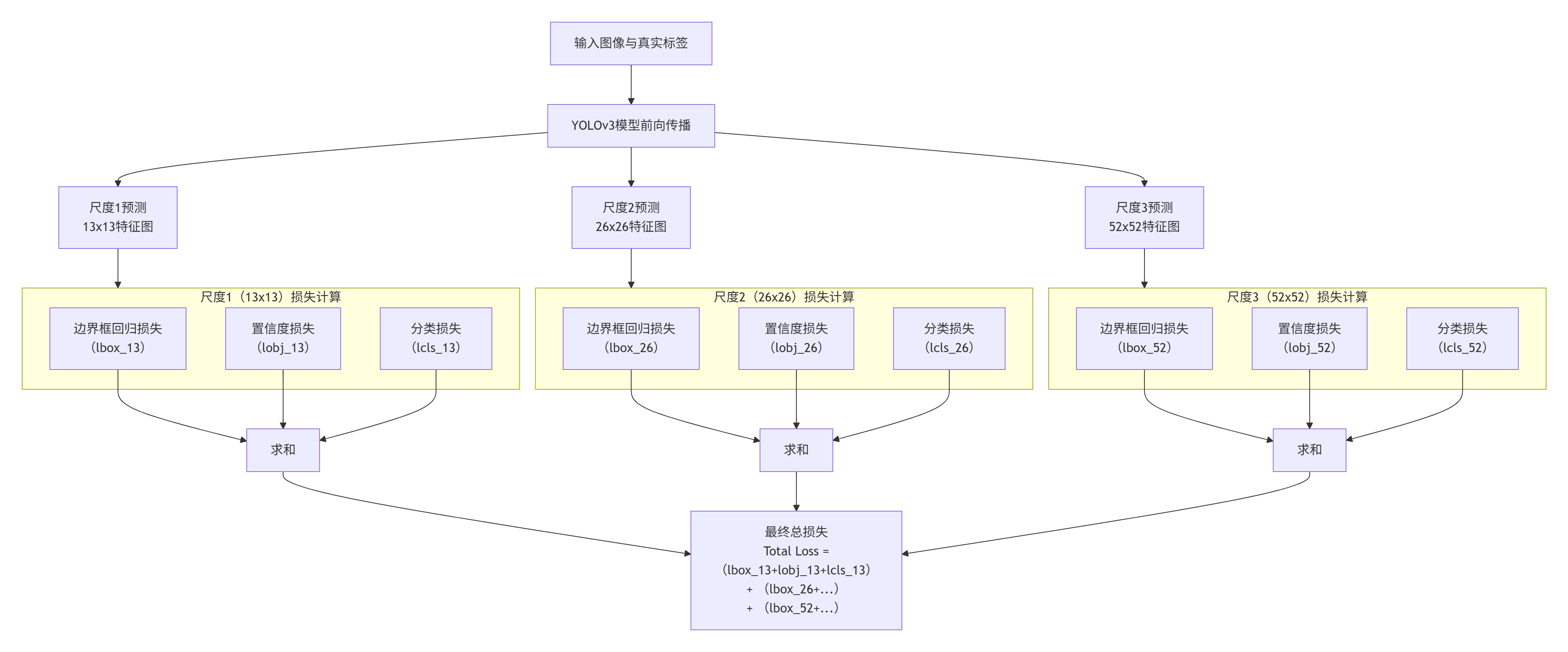
Taking the 13x13 scale feature map as an example, we explain the calculation pipeline for each component of the loss function.
First, let’s define and explain the sample types during YOLOv3 training. Generally speaking, YOLOv3 categorizes samples into three types when calculating the loss function during training: positive samples, negative samples, and ignored samples. Different types of samples are either used or not used to calculate different types of losses. As mentioned earlier, for the 13x13 resolution model output, a total of 13x13x3 = 507 prediction boxes are outputted. The determination of positive, negative, and ignored samples essentially involves evaluating and classifying these 507 prediction boxes, and then deciding based on the classification results whether they will be used for subsequent loss calculations.
- Positive Samples: For each ground truth box annotated in the training samples, the grid containing the center of the ground truth box is first identified. Then, among the three prediction boxes outputted by this grid, the one with the highest IOU with the ground truth box is selected as the positive sample. Thus, each ground truth box corresponds to one positive sample. Positive samples are used for all loss calculation types (bounding box, confidence, and classification).
- Ignored Samples: Those whose IOU with any ground truth box is greater than a specified threshold (e.g., 0.5), but which are not the positive sample for that ground truth box. Ignored samples do not participate in any loss calculations and thus have no impact on the final loss value.
- Negative Samples: Those whose IOU with all ground truth boxes is less than the specified threshold (e.g., 0.5), which essentially means all other samples excluding positive and ignored samples. Negative samples are used for confidence loss, but do not participate in bounding box and classification loss calculations.
Similar to previous YOLO versions, the YOLOv3 loss function also contains three parts: coordinate loss, confidence loss, and class loss.
For the calculation of coordinate loss, since only positive samples participate, the coordinate loss value is simply the loss between the coordinates of all positive samples and their corresponding ground truth boxes. Since the center coordinates, widths, and heights for all ground truth boxes and their corresponding positive samples are already known, calculating the coordinate loss is relatively straightforward:

Next is the calculation of confidence loss. YOLOv3 uses Binary Cross-Entropy (BCE) as the calculation function for confidence loss. The model outputs a confidence logit value for each prediction box. This value must be activated via the Sigmoid function, mapping it to the $(0, 1)$ interval to serve as the confidence score $\hat{C}$ representing the probability of containing an object. The confidence loss for a single prediction box is then calculated using the following formula, and summing the confidence losses of all prediction boxes yields the total confidence loss:
$$ L = - [ C * log(\hat C ) + (1 - C) * log(1 - \hat C) ] $$
As mentioned previously, confidence loss calculations consider positive and negative samples, while ignoring ignored samples.
- For positive samples ($C = 1$), the confidence loss simplifies to $-log(\hat{C})$. This means that the closer the model’s prediction $\hat{C}$ is to 1, the smaller the loss.
- For negative samples ($C = 0$), the loss simplifies to $-log(1 - \hat{C})$. This means that the closer the model’s prediction $\hat{C}$ is to 0, the smaller the loss.
Finally, we have the calculation of classification loss. The logic for calculating classification loss is largely identical to that of confidence loss, both employing Binary Cross-Entropy (BCE). However, only positive samples participate in the calculation of classification loss. Similarly, the model outputs a raw logit vector containing information for all classes for each prediction box. The length of this vector equals the number of classes in the dataset (e.g., 80 classes for the COCO dataset). These raw logit values must be activated via the Sigmoid function, mapping them to the $(0, 1)$ interval to serve as the parameter $P_{class}$ for classification loss calculation.
- Note that YOLOv3 allows class predictions where a single box can belong to multiple classes simultaneously (e.g., both “person” and “man” labels).
The classification loss for this positive sample across all classes is then calculated using the following formula, and summing the class losses of all positive samples yields the total classification loss:
$$ L_{class} = - Σ [ T_{class} * log(P_{class}) + (1 - T_{class}) * log(1 - P_{class}) ] $$