An Interpretation of the YOLOv3 Model Network Architecture
- 17 Oct, 2025
This article provides a detailed summary of the overall architecture of the YOLOv3 model, including its backbone network Darknet-53, the concept of Feature Pyramid Networks (FPN), and the design principles and implementation theory of multi-scale feature map detection heads.
The Brand-New Backbone Network: DarkNet-53
Starting from YOLOv2, the authors of the YOLO series designed a dedicated backbone network named Darknet. The backbone network used in YOLOv2 was DarkNet-19 (refer to Interpretation of YOLOv2 Model Network Architecture for the network architecture design of the YOLOv2 module), meaning the network structure contained a total of 19 convolutional layers. By the time of YOLOv3, the structural design of DarkNet drew inspiration from ResNet’s residual network structure—which had already become a mainstream design philosophy in the industry—and introduced DarkNet-53 as the backbone network for YOLOv3.
- For details regarding ResNet’s residual network structure, please refer to the article Learning Classical CNN Network Model Architectures: ResNet.
In the design of DarkNet-53, the convolutional layers still adopt the CBL combination structure used in Darknet-19: Convolution + BN (Batch Normalization) + LeakyReLU activation function. Darknet-53 contains 53 convolutional layers, from which it derives its name.

When performing spatial downsampling on feature maps, unlike DarkNet-19 which uses max-pooling layers, DarkNet-53 universally adopts $3 \times 3$ convolutional layers with a stride of 2 (stride=2). This approach reduces the feature map dimensions while preserving more spatial information. Therefore, the entire Darknet-53 network structure does not contain the MaxPool layers commonly found in traditional convolutional networks; all spatial downsampling operations on feature maps are handled by $3 \times 3$ convolutions with a stride of 2.
Furthermore, as mentioned above, the network design of Darknet-53 draws inspiration from the residual block design philosophy of ResNet. The residual block structure used in the Darknet-53 network is illustrated in the figure below. The input and output of the residual block are completely identical in feature map dimensions and channel counts. Internally, the block consists of a sequence of stacked $1 \times 1$ and $3 \times 3$ convolutional blocks, after which the output is added to the input to achieve a residual connection.
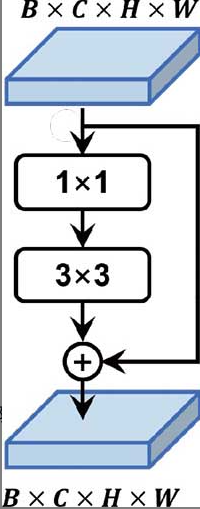
Similar to ResNet, the majority of the Darknet-53 network is essentially a stack of residual blocks. The figure below compares the YOLOv2 backbone network (Darknet-19) and the YOLOv3 backbone network (Darknet-53). As can be seen, the downsampling operations in Darknet-19 all use traditional max-pooling layers, whereas those in Darknet-53 exclusively use $3 \times 3$ convolutions with a stride of 2.
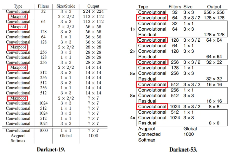
The network structure of Darknet-53 is constructed by repeatedly stacking the residual blocks described above. Overall, based on the feature map dimensions at various layers, Darknet-53 can be divided into 5 parts (as circled on the right side of the figure above). The number of residual blocks contained in each of the five parts from first to last are 1, 2, 8, 8, and 4, respectively. The dimensions and channel counts of the input and output feature maps remain consistent within each part, and a $3 \times 3$ convolution with a stride of 2 is used between parts to reduce the feature map dimensions. This “1-2-8-8-4” stacking configuration has also become one of the standard design paradigms for subsequent YOLO frameworks.
Darknet-53 is fundamentally still a network for image feature extraction and category classification. Therefore, it ultimately still employs global average pooling combined with fully connected layers and Softmax to output recognition and classification results for the ImageNet dataset. Of course, when used as the backbone network for the YOLOv3 model, the global average pooling and subsequent layers are removed, retaining only the preceding feature extraction portion to output feature maps at different stages for object detection.
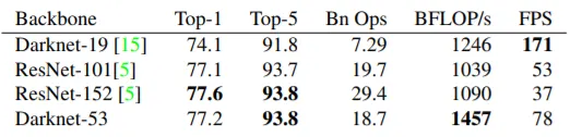
Below is a comparison of the Darknet-53 network with architectures such as Darknet-19, ResNet-101, and ResNet-152 in terms of metrics like recognition accuracy and running speed. As can be seen, although the speed of Darknet-53 is lower than that of Darknet-19, it still achieves real-time performance, and its recognition accuracy is significantly improved.
Feature Pyramids and Feature Fusion
The Feature Pyramid Network (FPN) originates from another object detection network architecture, SSD. The underlying design philosophy is that as the neural network goes deeper and downsampling operations increase, the feature maps output at each layer contain different information: shallow feature maps have higher resolution and thus contain more positional information, but have smaller receptive fields due to fewer downsampling operations, making object category recognition more difficult; conversely, deep feature maps have lower resolution, where object positions and details are lost during progressive downsampling, but because their receptive fields are relatively larger, their performance in identifying and detecting large objects is better. Therefore, to address this inherent contradiction, a natural solution emerges: comprehensively combining shallow and deep features, where shallow features are responsible for detecting smaller objects, and deep features are responsible for detecting larger objects.
- The larger the feature map resolution, the richer the positional details, but due to an excessively small receptive field, determining the object category becomes more difficult.
- The smaller the feature map resolution, the greater the loss of object positional information during multi-level downsampling, but as the receptive field gradually increases, it becomes easier to determine the category of the target being detected (especially large-scale objects).
The following figure illustrates the structure of a feature pyramid: the feature extraction network on the left outputs feature data of three resolutions and dimensions, while the detection network on the right performs detection and recognition for large, medium, and small objects respectively.
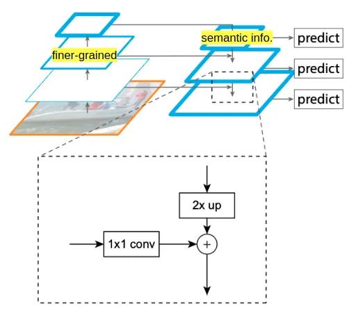
To detect large-scale objects, it is sufficient to use only the feature information with the smallest resolution (the top-layer prediction output in the figure above). This is because for larger objects, although the positional information loss in low-resolution feature maps is relatively high, it is sufficient for localizing large objects. Moreover, low-resolution feature maps have larger receptive fields, making it easier to distinguish object categories, thus eliminating the need to rely on high-resolution feature information.
For detecting smaller objects, however, one must use not only the higher-resolution feature information output by the feature extraction network (utilizing the rich positional information contained within to accurately localize small objects) but also the lower-resolution feature information (to assist in determining and localizing the object category). Therefore, it is necessary to fuse low-resolution feature information with high-resolution feature information to achieve accurate localization and category determination for small and medium-sized objects.
The next question is: how are feature maps of different resolutions fused? The answer is to apply spatial upsampling (Upsample, i.e., $2\times$ up in the figure above) to the low-resolution feature maps output by the deep network to raise their resolution to match that of the shallow features, and then fuse them with the shallow-resolution feature maps. This process primarily involves two operations: spatial upsampling (Upsample) and feature map fusion (Concat).
The fusion of the $13 \times 13$ resolution feature map and the $26 \times 26$ resolution feature map in the YOLOv3 model is used below to explain the Upsample and Concat operations:
Upsampleoperation: Based on the $13 \times 13$ resolution feature map, $2 \times 2$ interpolation is performed using nearest-neighbor interpolation. Every $13 \times 13$ resolution feature map is upsampled via this interpolation method into a $26 \times 26$ resolution feature map.Concatoperation: After being upsampled via theUpsampleoperation, the aforementioned feature map matches the $26 \times 26$ resolution. This yields two sets of $26 \times 26$ resolution feature maps, which are then simply concatenated end-to-end along the channel axis.
The fusion processing and output workflow for feature maps of different resolutions are illustrated in the figure below:
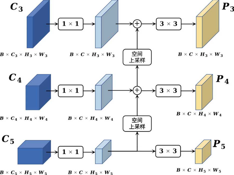
The YOLOv3 Architecture Diagram
Based on the preceding understanding of the backbone network Darknet-53 and the multi-branch feature map output structure of the feature pyramid, learning the network structure of YOLOv3 becomes much easier:
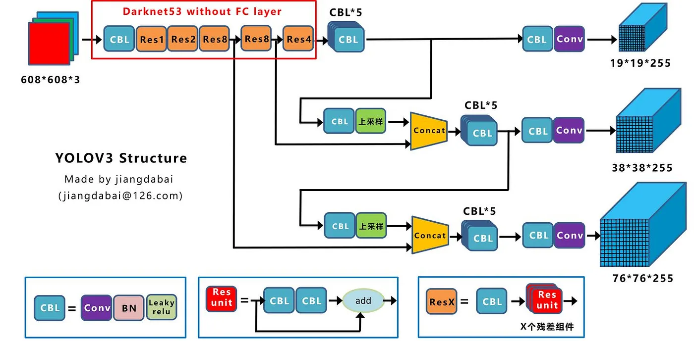
The top-left corner of the figure above shows Darknet-53, the backbone network of YOLOv3, with the global average pooling and classification fully connected layers removed. Feature maps downsampled by factors of 8, 16, and 32 are output from the third, fourth, and fifth residual block groups of the backbone network, respectively.
- For an input image resolution of $608 \times 608$, the feature map resolutions output by these three parts are $76 \times 76$, $38 \times 38$, and $19 \times 19$, respectively.
- For an input image resolution of $416 \times 416$, which was more common in object detection scenarios at the time, the resolutions of these three feature map branches are $52 \times 52$, $26 \times 26$, and $13 \times 13$, respectively.
The right half of the figure above represents the feature detection portion based on FPN theory, taking feature maps of three different resolutions as inputs. Upsampling and Concat operations are performed at different stages, ultimately outputting detection networks with varying grid densities: denser grids are better suited for detecting small and dense objects, while sparser grids are better suited for detecting large and sparse objects.
References
- “YOLO Object Detection” by Jianhua Yang, Ruifeng Li, Chapter 7: YOLOv3
- YOLOv3 Detailed Interpretation. YOLOv3… | by Steven Meng | Medium
- “Deep Learning PyTorch Object Detection in Action” by Hongyi Dong, 6.3 Multi-scale and Feature Fusion YOLOv3
- YOLOv3 — You Only Look Once (Object Detection) | by Moris | Computer Vision Note | Medium