Summary of YOLOv2 Features: Evolution from YOLOv1
- 15 Oct, 2025
This article provides a comprehensive summary of the features evolved in YOLOv2 based on YOLOv1, explaining the characteristics and working logic that improved various model metrics during its evolution.
Built upon the design foundation of YOLOv1, YOLOv2 introduced multiple adjustments and optimizations in model design and training. Its mAP on the VOC2007 dataset increased dramatically from 63.4% to 78.6%, while retaining the one-stage design of YOLOv1 for object detection and class recognition. It maintains a very fast inference speed while being capable of recognizing more object categories.
- For the concept and calculation logic of the mAP metric, please refer to Detailed Explanation of Evaluation Metrics for Object Detection Models: mAP, Recall, Precision.
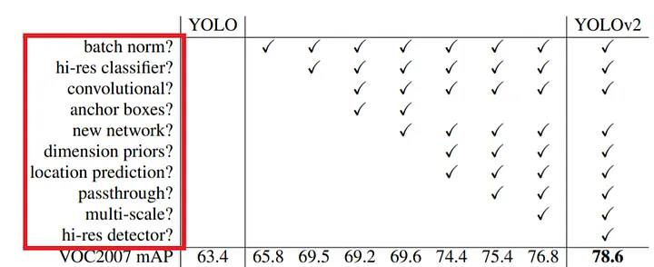
The following figure summarizes the complete list of improvements made in YOLOv2 compared to YOLOv1. Each of these items will be elaborated on in this article:
Batch Norm
YOLOv2 adds batch normalization after every convolutional layer in the model. Thus, the previous configuration of convolution + LeakyReLU activation function has been upgraded to a CBL block consisting of convolution + batch normalization + LeakyReLU activation function.
Specific details are thoroughly described in the article Interpretation of YOLOv2 Model Network Architecture.

With the addition of the BN layer, YOLOv2 achieved its first performance boost. On the VOC2007 test set, its mAP improved from the original 63.4% to 65.8%.
Hi-res Classifier
Because the ImageNet dataset contains a massive amount of annotated image data, most object detection algorithms first pre-train the backbone network based on the ImageNet dataset, using these pre-trained parameters as the initial parameters for the backbone network—a technique known as Image Pretraining.
However, during the pre-training process based on the above technique, the input image size received by the backbone network is 224x224. For object detection applications, this small resolution easily leads to the loss of details for small objects, creating difficulties for subsequent detection stages. Therefore, in the design of YOLOv2, a strategy was adopted where the model is first pre-trained on the ImageNet dataset at a 224x224 resolution. Once pre-training is complete, a model fine-tuning stage is added: the network continues training at a 448x448 resolution using the pre-trained parameters to adapt to higher-resolution images.
Specifically, the pre-training workflow of the YOLOv2 model is as follows:
- First, train the network from scratch on the ImageNet dataset using a 224x224 resolution for approximately 160 epochs.
- Then, adjust the model input to 448x448 and continue training on the ImageNet dataset for another 10 epochs.
Under this strategy, YOLOv1’s performance improved once again: mAP increased from 65.8% to 69.5%.
Why not train the network from scratch directly at the 448x448 resolution, but instead pre-train at a small resolution of 224x224 followed by fine-tuning at a large resolution of 448x448? On one hand, scaling from 224x224 to 448x448 quadruples the resolution, which would significantly prolong model training time given the computing power available at the time. On the other hand, a 224x224 resolution was the standard input for classification networks back then, with a wealth of pre-trained weights and hyperparameter experience available for reference. Therefore, starting with a mature configuration as a warm-up followed by minor fine-tuning is the most reliable approach from an engineering perspective.
Fully Convolutional Network and Anchor Prior Box Mechanism
In terms of network architecture design, the biggest change in YOLOv2 compared to YOLOv1 is the removal of fully connected layers at the end of the network, replacing them with a fully convolutional network structure. For the specific network structure, refer to Interpretation of YOLOv2 Model Network Architecture.
In addition, drawing inspiration from the Faster R-CNN network, YOLOv2 introduces the Anchor prior box mechanism. During the image inference stage, the model only needs to learn the offsets required to map prior boxes to the dimensions of the target bounding boxes, rather than learning the complete dimension information of the entire target box from scratch, which makes training much easier. For a detailed summary of the Anchor prior box mechanism introduced in YOLOv2, refer to Detailed Explanation of the Anchor Mechanism in YOLOv2.
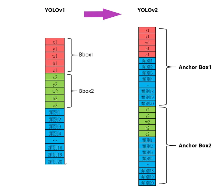
Based on the optimization of the model’s network structure and the introduction of Anchor boxes, the size of the feature map output by the backbone network is increased from YOLOv1’s scale to YOLOv2’s 13x13. $K$ Anchor boxes are placed in advance at each grid cell (in the YOLOv2 model, the default number of Anchor boxes is 5). This means the entire image can output $13 \times 13 \times K = 169K$ bounding boxes, and the prediction information for each bounding box is completely independent. Each bounding box has its own center coordinates $x$ and $y$, box width $w$ and height $h$, prediction confidence, and recognition probabilities for various categories (in the YOLOv1 model, two bounding boxes in a network shared the same class recognition probability, so each bounding box could actually only detect one object). Therefore, the bounding boxes output by the same grid cell in YOLOv2 are mutually independent, which resolves the missed detection problem that occurs when the centers of two objects fall within the same grid cell. The differences in output information between the YOLOv1 and YOLOv2 models are illustrated in the figure below:
Multi-Scale Training
Following the modification of the network structure to remove fully connected layers and adopt a fully convolutional network structure—containing only convolutional layers and max-pooling layers—the input resolution of the entire network is no longer restricted to 416x416 images; images of various different resolutions can be used. Consequently, during the training process, the input image size can be continuously changed to adapt to different resolutions and varying sizes of objects to be detected.
The backbone network (image feature extraction part) of the YOLOv2 model has a downsampling stride of 32, meaning the size of the feature map extracted by the feature extraction part is $1/32$ of the input image resolution. Therefore, the input resolution of the image needs to be a multiple of 32 (with a minimum size of 320x320 and a maximum size of 608x608). Thus, during the training process of the YOLOv2 model, every 10 epoch iterations, the model randomly selects a new image size from {320, 352, 384, 416, 448, 480, 512, 544, 576, 608} to serve as the image size for the subsequent 10 epochs of training, as shown in the figure below:
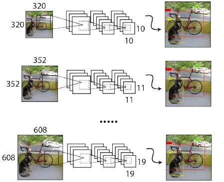
Practice has proven that this Multi-Scale Training strategy allows the same network to perform detection with higher accuracy on images of different resolutions, thereby enhancing the detection performance of the network.
References
- YOLOv2 Detailed Explanation. YOLOv2 is improved based on YOLOv1 using the methods in the red box above, in… | by Steven Meng | Medium
- “YOLO Object Detection” by Jianhua Yang, Ruifeng Li, Chapter 6: YOLOv2