Detailed Explanation of the Anchor Mechanism in YOLOv2
- 12 Oct, 2025
This article summarizes the origin, calculation, and training process of the Anchor mechanism introduced in YOLOv2—built upon Faster R-CNN’s theory for model grid prediction box design—in an attempt to provide a clearer understanding of the YOLOv2 model’s working principles.
The Concept of Anchor Boxes
First, let’s define an Anchor box: An anchor is a bounding box with pre-determined dimensions and aspect ratios placed fixedly within each image segmentation grid prior to training. Typically, the size and number of pre-placed bounding boxes are identical for every grid. During inference, based on the objects to be detected in the input image, the model predicts several offsets (such as center position offsets, width and height offsets) for each pre-placed bounding box, and then adjusts the pre-placed bounding box using these offsets to derive the final predicted bounding box. Therefore, the bounding boxes pre-placed at each grid are anchor boxes; their essence is to provide a size estimation for the bounding boxes, and then use the offsets calculated by the model during inference to adjust their position and size, thereby obtaining the final bounding box dimensions.
You can directly visualize what an anchor box is from the image below: the image divides the entire picture into 7x7 grids, just like YOLOv1, and three anchor boxes of different sizes and proportions are pre-placed on each grid. For demonstration convenience, the diagram only shows one set of anchor boxes for every six grids; in reality, every grid has a set of anchor boxes, but drawing all of them would make it too dense and less intuitive for demonstration.
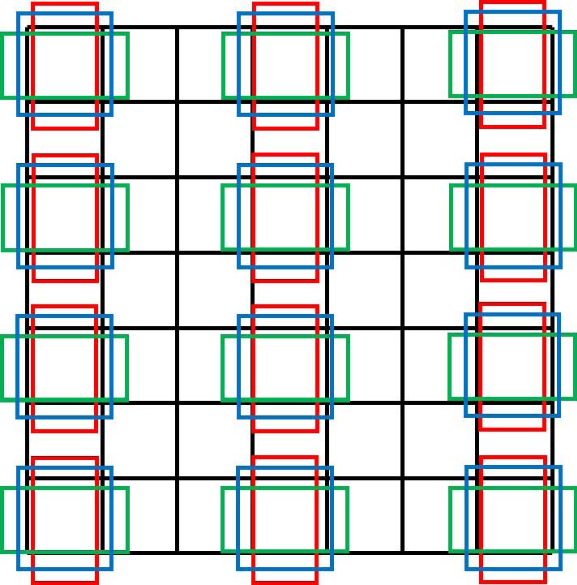
From the concept of anchor boxes, the YOLOv1 version did not have a design for pre-placing anchor boxes. Instead, it simply defined two boxes for each grid, and the center positions and sizes of both boxes had to be predicted by the model during the inference process based on the input image. Thus, from this perspective, YOLOv1 is a typical Anchor-free model.
The design of pre-setting anchor boxes in each grid originally stems from another object detection model: Faster R-CNN. Faster R-CNN is a two-stage object detection model that localizes objects in the first stage and recognizes object categories in the second stage. Its approach to object localization and detection is similar to YOLOv1—dividing the input image into multiple grids and searching for objects grid by grid. However, the first stage of Faster R-CNN only identifies which grids contain objects without caring about their categories, and the second stage subsequently identifies the specific categories of the detected objects. In contrast, YOLOv1 localizes objects and recognizes their categories simultaneously. This is the biggest difference in object searching and prediction workflows between Faster R-CNN and the various YOLO versions.
For the Faster R-CNN model, the input is first divided into multiple grids, and then $k$ anchor boxes with different sizes and aspect ratios are preset for each grid (as shown in the image above). YOLOv2 also adopted this preset anchor box mechanism, significantly improving the model’s mAP metric. With the addition of anchor boxes, during the inference phase, the model no longer needs to directly predict the size and coordinates of the target object from scratch; instead, it only needs to predict the offset from the anchor box to the ground truth object, thereby reducing the prediction difficulty.
The K-Means Clustering Algorithm for YOLOv2 Anchor Boxes
The question is, how do we determine how many anchor boxes should be placed in each grid, and how should the size and aspect ratio of each anchor box be decided? For the Faster R-CNN model, parameters such as the number and size of anchor boxes are manually set as hyperparameters. Such a design makes it difficult to ensure that the manually specified anchor box parameters match the dataset, leading to unstable network performance across inputs from different datasets.
To address this issue, the approach taken by the YOLOv2 model is to use the k-means clustering algorithm to extract the most suitable anchor boxes from a designated dataset.
First, all ground truth (GT) bounding boxes from the images in the entire training set are extracted and resized to a uniform input dimension (416x416): the algorithm only cares about the width and height information of the ground truth boxes, which is the aspect ratio.
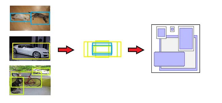
Traditional K-means clustering algorithms use Euclidean distance during clustering calculations. However, this means that larger anchor boxes would produce more errors compared to smaller ones, causing the clustering results to bias. The goal of YOLOv2’s clustering calculation is to ensure that the pre-selected anchor box sizes have a larger IoU with their closest ground truth boxes, regardless of the absolute scale of the anchor and ground truth boxes. Therefore, the YOLOv2 model defines the following distance formula to execute the clustering algorithm:
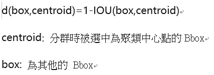
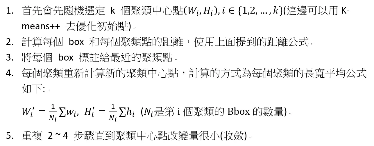
Randomly pick 5 initial anchor boxes from the list of all extracted ground truth boxes, and execute the k-means clustering algorithm described below:
- Based on the clustering formula described above, calculate the
distvalue between all ground truth boxes in the dataset and the 5 anchor boxes. Each ground truth box is grouped into the cluster of the anchor box with which it shares the maximumdistvalue. Repeat this logic until all ground truth boxes are processed and divided into 5 clusters based on the anchor boxes. - Perform the following calculations on the list of ground truth boxes contained in each cluster:
- Take the width of all ground truth boxes in the cluster (the resolution of the ground truth boxes was previously uniformly resized to 416x416), calculate the geometric mean of all widths, and replace the width of that cluster’s anchor box with this calculated geometric mean.
- Similarly, take the height of all ground truth boxes, calculate the geometric mean of all heights, and replace the height of that cluster’s anchor box with this calculated geometric mean.
- After the above operations, 5 new anchor box
(width, height)pairs are obtained. - Then, re-execute the clustering algorithm from scratch based on these 5 new anchor boxes to obtain updated anchor box
(width, height)pairs. Through such iterative calculations, the width and height of the new anchor boxes eventually stabilize. These are the final anchor boxes automatically generated by the algorithm based on the dataset.
The execution flow of the entire k-means clustering algorithm above can be simplified into the following diagram:
Once the width and height parameters of the 5 anchor boxes are calculated based on the above logic and process, they can be written into the configuration (cfg) file of the YOLOv2 model in order of their surface area. Subsequently, during the model’s training and inference processes, 5 sets of anchor boxes with these length-width ratios will be placed in each grid to detect objects in the image.
However, the severe limitations of this algorithm are also apparent from the calculation logic: the anchor boxes selected through this algorithm are based on a specific dataset and will therefore only perform well on that dataset. If a new dataset has significant differences in the sizes of target objects compared to the training dataset, the initially chosen anchor boxes will become unsuitable.
Anchor-Based Bounding Box Prediction
Following the clustering calculation of the anchor boxes described above, 5 sets of anchor boxes with determined aspect ratios are obtained before the model begins formal training. With this prior dimensional information of the anchor bounding boxes during training, the network no longer needs to learn the width and height of the entire target box from scratch.
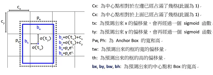
Assume the dimensions of a predefined anchor box are $p_w$ and $p_h$, the top-left coordinate position of the grid containing the center of the target object is $grid_x, grid_y$, the center offset output by network inference is $(t_x, t_y)$, and the width and height offsets output by the network are $(t_w, t_h)$. Then, the YOLOv2 model calculates the center coordinates and bounding box of the target object using the following formulas:
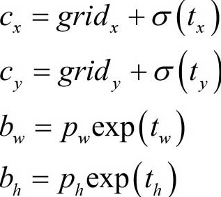
The center offset $(t_x, t_y)$ predicted and output by the YOLOv2 model is relative to the top-left corner of its containing grid. Furthermore, when calculating the actual center position, a Sigmoid function is used to constrain the offsets added to $grid_x, grid_y$ to be between 0 and 1. This ensures that the center point of the predicted bounding box remains inside the grid and does not drift significantly outside of it.
You can understand the formulas above with the help of the following diagram: the dashed box represents the anchor box, and the blue box represents the bounding box calculated from the model’s prediction output.
References
- YOLO Object Detection, Yang Jianhua, Li Ruifeng, Chapter 6: YOLOv2
- PyTorch Deep Learning Object Detection in Action, Dong Hongyi, Section 6.2 Anchor-Dependent: YOLOv2
- YOLOv2 Detailed Explanation. YOLOv2 is improved upon YOLOv1 by using the methods in the red box above, at… | by Steven Meng | Medium