An Interpretation of the Loss Function and Training Process in YOLOv1
- 08 Oct, 2025
This article summarizes the training positive sample labeling method, loss function, and the complete training process of the YOLOv1 model, laying a solid foundation for understanding the processing workflows of subsequent YOLO versions.
Labeling of Positive Training Samples in YOLOv1
As summarized in the article Detailed Interpretation of YOLOv1 Output Information and NMS Filtering Algorithm, the object detection logic of YOLOv1 is that if the center point of an object falls within a specific grid cell, that grid cell is responsible for detecting the object. This means that when constructing training samples for YOLOv1, only the grid cell containing the center point of the target object is considered to contain an object.
This is illustrated in the figure below:
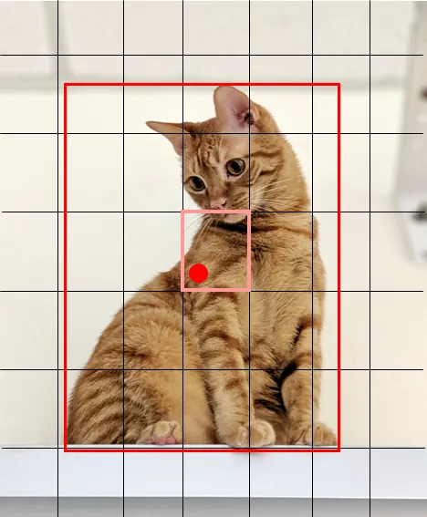
Although the bounding box for the kitten in the figure spans as many as 24 grid cells, because the center of this bounding box falls within the pink grid cell, only the pink grid cell is labeled as containing an object when generating the training sample for this image in YOLOv1. The detection confidence for this grid cell is close to 1, while all other grid cells are considered to contain no object, with a detection confidence close to 0.
Grid cells containing objects are labeled as positive sample candidate regions. That is, during the training process, positive training samples are derived exclusively from the predictions at these grid cells, whereas predictions from all other regions serve as negative samples for that target.
Interpretation of the YOLOv1 Loss Function
Overall, the calculation of the YOLOv1 loss function consists of three main components:
- Coordinate Loss ($x, y, w, h$): Evaluates how closely the bounding boxes predicted by the model fit the ground truth boxes of the training samples.
- Confidence Loss: Measures the degree of alignment between the confidence value of each predicted box output by the model and whether that box actually contains the target object to be detected.
- Classification Loss: Determines whether the category predictions output by the model match the labeled classification of the training samples.
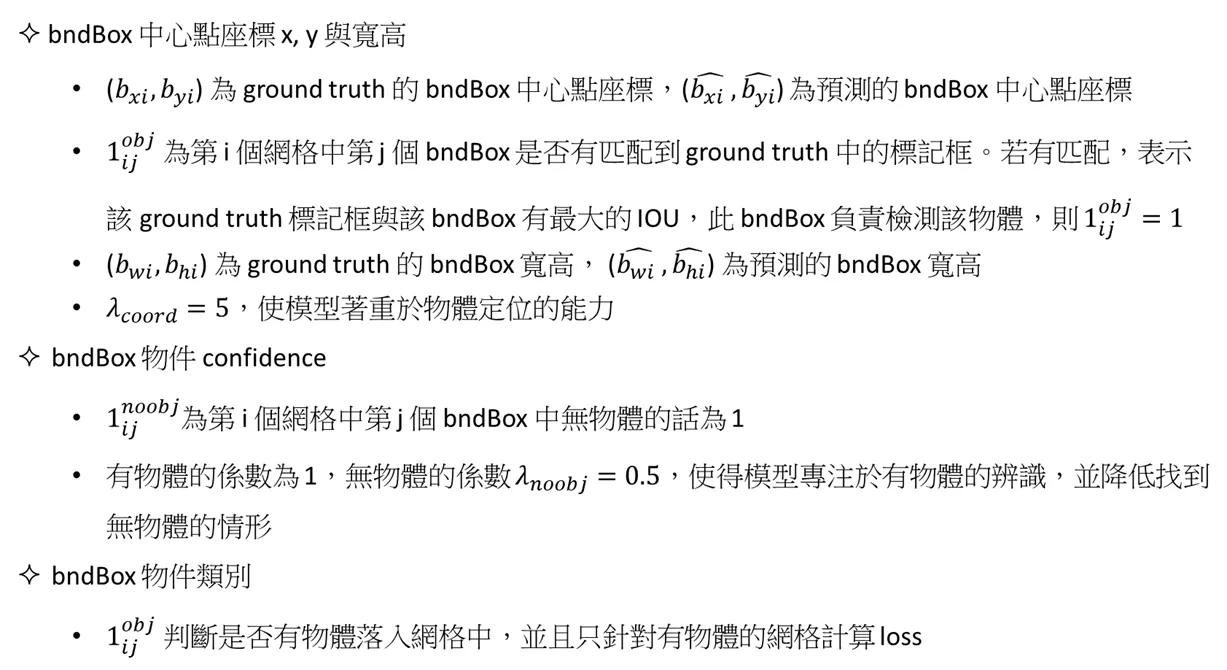
The figure below shows the meanings of various parameters used in the loss function calculation:
The figure below shows the calculation formula of the YOLOv1 loss function:
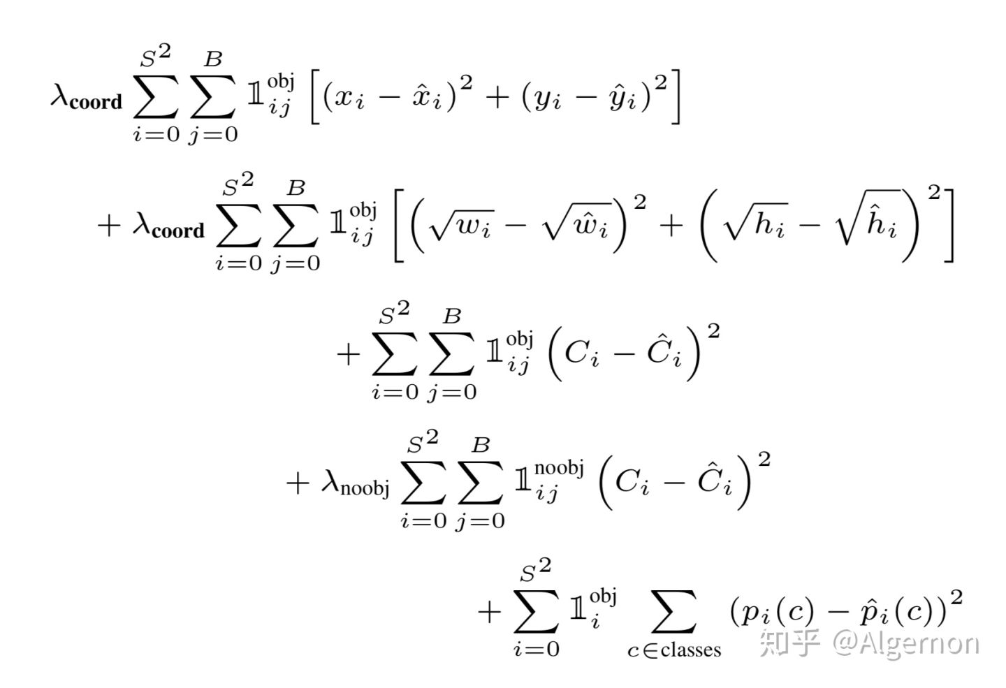
The first two rows of the YOLOv1 loss function represent the loss for the coordinate parameters of the predicted bounding boxes, the third and fourth rows represent the confidence loss for both positive and negative sample bounding boxes, and the last row represents the classification loss at the positive samples.
Although the calculation logic of the loss function above looks complex, the actual computation logic is quite intuitive. It can be broken down into three parts for detailed explanation.
Coordinate Loss
The key to calculating the coordinate loss is understanding the meaning of $1_{ij}^{obj}$:
- For each ground truth box of a training sample, first locate the grid cell where the center of this ground truth box falls. Then, calculate the IOU between the two predicted boxes output by this grid cell and the ground truth box, and set the $1_{ij}^{obj}$ value of the predicted box with the larger IOU to 1, while setting the $1_{ij}^{obj}$ value of the other predicted box to 0.
- In this case, effectively, exactly one predicted box with a $1_{ij}^{obj}$ value of 1 is found for each ground truth box in the training sample.
The logic above identifies the responsible predicted box corresponding to each ground truth box in the training sample. Next, following the respective formulas, the loss values for the center coordinates, width, and height between the ground truth box and the responsible predicted box are calculated. The sum of these two loss values gives the total coordinate loss.
As seen from the loss function formula above, the coordinate loss value is also multiplied by a coefficient $\lambda_{\text{coord}} = 5$. This increases the weight of the bounding box localization precision loss in the overall loss, prioritizing more accurate localization of the predicted boxes.
Confidence Loss
The calculation of confidence loss consists of two parts: the loss for responsible predicted boxes and the loss for non-responsible predicted boxes.
Loss for responsible predicted boxes: For each ground truth box of the training sample, follow the same steps as the coordinate loss calculation above to find the corresponding responsible predicted box. Each ground truth box has only one responsible predicted box. Then, calculate the confidence loss between the ground truth box and the responsible predicted box. Here, the target confidence of the ground truth box is 1, and the confidence of the responsible predicted box is the model’s confidence output value for this predicted box.
Loss for non-responsible predicted boxes: The logic for non-responsible predicted boxes is simple. Among the 98 predicted boxes output by the model, apart from the aforementioned responsible predicted box, the remaining 97 boxes are all non-responsible predicted boxes.
Calculate the loss values for the responsible and non-responsible predicted boxes separately using the formulas above. Then, multiply the loss of the non-responsible predicted boxes by $0.5$ to suppress the impact of background boxes on the loss values of the true predicted boxes. Summing these two gives the total confidence loss.
Classification Loss
The classification loss is calculated exclusively for the responsible predicted boxes; the classification loss for all other predicted boxes is 0.
For each responsible predicted box, calculate the loss between its 20 class recognition probabilities and the ground truth class of the training sample. It is worth noting that the class of the ground truth box is provided as a 20-dimensional label in one-hot format (only one class is 1, and all others are 0). Therefore, the classification loss is the squared difference between the 20 class recognition probabilities corresponding to each responsible predicted box and the 20-dimensional probability labels of the one-hot ground truth box.
References
- “YOLO Object Detection” by Jianhua Yang, Ruifeng Li, Chapter 3: YOLOv1
- YOLO Evolution — 1. The previous article mentioned YOLO’s approach and how to train it; this article explains YOLO in even more detail… | by Ching-I | Ching-I’s Reading Notes | Medium