Detailed Explanation of YOLOv1 Output Information and NMS Filtering Algorithm
- 07 Oct, 2025
The network architecture of the YOLOv1 model has already been explained in great detail in the article [[Detailed Interpretation of the YOLOv1 Model Network Architecture]]. Below is the architecture diagram of the YOLOv1 network:
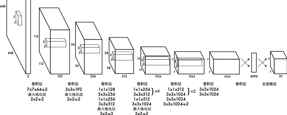
As can be seen from the architecture diagram above, compared to various classic convolutional neural network models used for image classification, the network structure of YOLOv1 does not introduce particularly groundbreaking innovations. It still extracts features from images through repeated convolution and pooling operations in the first half of the network, and performs category recognition and localization using two consecutive fully connected layers in the second half. However, compared to other networks, the essence of the YOLOv1 architecture lies in its final 7x7x30 output interpretation, the training of model parameters, and the design of its loss function evaluation.
YOLOv1 Model Output Information
The output of YOLOv1 is a 3D tensor of size 7x7x30. This can be conceptualized as dividing the input image of 448x448 resolution into a 7x7 grid. The model searches for the center point of the target object to be recognized, its bounding box, confidence score, and object category within each grid cell. Each grid cell represents these detected items using a 30-element vector.
As shown in the figure below, each grid cell outputs the information for two bounding boxes. The information for each box includes the coordinates of the detected object’s center point (relative to the top-left corner of the grid cell), the width and height of the detected object (expressed as ratios relative to the entire image size of 448x448), and the confidence score of this detection box.
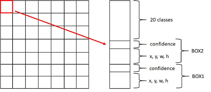
It is important to note that YOLOv1’s logic for detecting objects in an image is: if the center point of an object falls within a certain grid cell, that grid cell is responsible for detecting and outputting the corresponding bounding box and other information for that object. Therefore, in the box information output by each grid cell, $x$ and $y$ represent the position of the center point of the target object relative to the top-left corner of the current grid cell, while $w$ and $h$ represent the width and height of the bounding box predicted by this grid cell relative to the entire input image resolution.
Each box has a confidence parameter, which is used to characterize the probability that the current box actually contains the target object. If the box contains the center point of a target object, this confidence parameter will be relatively high, approaching 1. Conversely, if the box does not contain the center point of any target object, its confidence will approach 0, allowing it to be filtered out in subsequent filtering algorithms.
The 20 classes are used to represent the final recognition probabilities for various target object categories. For the VOC dataset, it supports the detection and recognition of 20 categories. If the COCO dataset is used, the number of categories output by each grid cell needs to be modified to the recognition probabilities of 80 categories.
Two Boxes, One Set of Category Recognition Probabilities?
From the output information of each grid cell of the YOLOv1 model summarized above, we can see that the output of each grid cell contains the information of two predicted boxes, along with a single set of recognition probabilities for the target objects. So, if a grid cell happens to contain the centers of two target objects, which object do these category recognition probabilities actually represent?
The answer is: in this case, a missed detection will definitely occur. This is also the fundamental reason why YOLOv1’s recall rate drops sharply in dense, small-target scenarios, and it is the motivation for subsequent versions (starting from YOLOv2) to introduce anchors, refining the “responsible detection unit” from grid cells to “grid + anchor” or even “pixel” levels.
Let’s understand this concept based on the figure below:
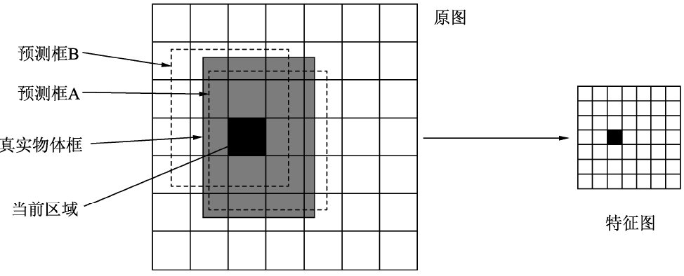
For the two boxes output by each grid cell, the grid cell will only mark the box that best matches the actual target object (specifically measured by the IOU metric) as a positive sample during output. In the figure above, the bounding box of the actual object is the light gray box, and the matching degree of predicted box A is much better than that of predicted box B. Therefore, in the output of this grid cell, the confidence score of predicted box A will be relatively high, while the confidence score of predicted box B will be suppressed to a lower value. The category information contained in this grid will correspond to the category recognition probability of the image region enclosed by predicted box A.
Thus, the entire input image in YOLOv1 is divided into 7x7 grid cells, and each grid cell outputs 2 boxes. At first glance, it seems that YOLOv1 can achieve a maximum detection of $7 \times 7 \times 2 = 98$ objects. However, in reality, each grid cell can output at most one box and its corresponding recognition category, so the entire image can recognize a maximum of only 49 independent objects. In other words: The two boxes output by each grid cell are not intended to detect two objects within a single grid cell; rather, after an object is detected in a grid cell, the two boxes provide an either-or option, allowing the model to select the best-matching box to locate its position.
NMS
NMS stands for Non-Maximum Suppression. As the name suggests, it is an algorithm that suppresses bounding boxes that are not the maximum, where “suppression” typically means filtering out redundant bounding boxes for the same detected object.
As mentioned above, for each image input into the YOLOv1 model for inference and detection, the model outputs $7 \times 7 \times 2 = 98$ predicted boxes via the 7x7x30 3D tensor. These 98 predicted boxes must still go through the NMS algorithm filtering process to truly output the final detection results; otherwise, a single object might have multiple output detection boxes.
The basic execution logic of the NMS algorithm: Use bounding boxes with high scores to suppress overlapping bounding boxes with low scores.
The execution of the NMS algorithm is processed independently according to the supported categories. Each NMS operation yields the final detection boxes for a single category. Although the calculation logic is identical for different categories, combining the final detection boxes of all categories together at the end yields the final detection results of the model.
Step 0: For a specific category, multiply the confidence of the box by the recognition probability of this category to obtain the score of this box for this category. Since the model outputs 98 boxes, each category will have 98 scores.
Step 1: Compare the 98 scores of this category with the NMS detection threshold (e.g., 0.2). Boxes with scores lower than this threshold are deleted, and only boxes greater than the threshold are kept in the candidate list.
Step 2: Sort all boxes in the candidate list in descending order based on their scores, and directly move the box with the highest score in the candidate list into the detection output for that category.
Step 3: Calculate the IOU (Intersection over Union) between the box with the highest score and all other boxes in the candidate list. When the calculated IOU value is greater than the IOU threshold (typically 0.5), it indicates that the two boxes are detecting the same target. In this case, the box with the lower score is removed from the candidate list.
Step 4: Remove the box with the highest score from the current candidate list.
Repeat steps 2 to 4 above until the candidate list of boxes is empty. At this point, the detection output results for this category are obtained. After performing the above steps for all 20 categories, combining the detection output results of all categories gives the final detection output of the model.
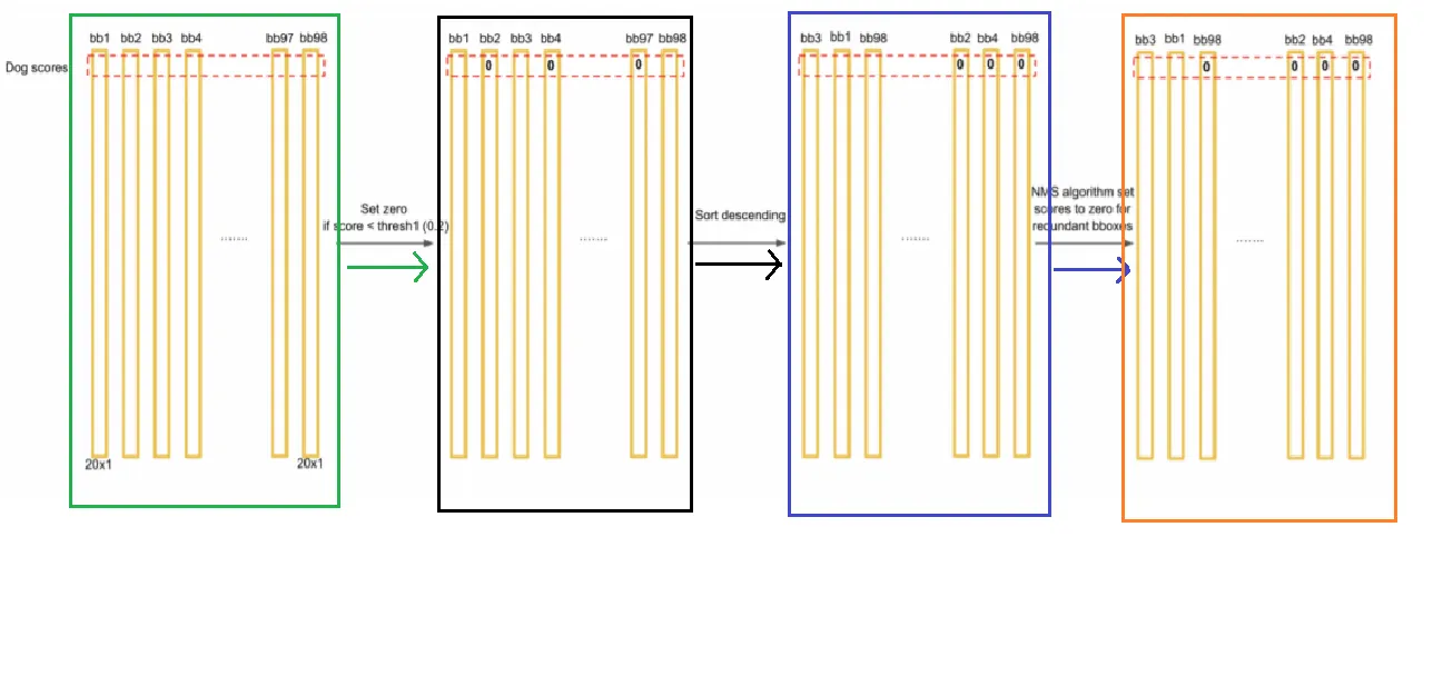
The figure above illustrates the NMS algorithm filtering process for the “dog” category.
- First, for the dog category, multiply the confidence score of each box by the recognition probability of the dog category in its corresponding grid cell to obtain 98 scores.
- Compare these 98 scores against the threshold of 0.2, delete boxes with scores less than 0.2, and put the remaining boxes into a candidate list.
- Sort the boxes in the candidate list in descending order based on their scores. The box with the highest score is directly added to the detection output for the dog category. Simultaneously, execute the NMS algorithm described above: each time, place the box with the highest score into the output list for that category, and eliminate other boxes that heavily overlap with this box using IOU (to prevent multiple detection boxes for a single detected object) until the entire candidate list of boxes is emptied.
References
- “Deep Learning with PyTorch Object Detection in Action”, Section 6.1 Anchor-Free Prediction YOLOv1
- All of the start: YOLOv1. YOLO: you only look once. | by John Shen | Medium
- YOLOv1 Detailed Interpretation. Design Concept: | by Steven Meng | Medium