Learning Classical CNN Network Architectures: ResNet
- 30 Sep, 2025
The ResNet network architecture was proposed by Kaiming He and other researchers from Microsoft Research Asia in 2015 in their paper Deep Residual Learning for Image Recognition. It won first place in multiple tasks such as classification, detection, and localization in the 2015 ImageNet image recognition competition. The core contribution of this model lies in solving the training bottleneck of deep networks, making it possible to train networks with hundreds or even thousands of layers, which greatly advanced the development of computer vision.
Training Challenges of Deep Networks
Before the ResNet network architecture was introduced, researchers discovered during the research and training of deep neural networks that:
- Theoretically, the deeper the network structure and the more layers it has, the stronger its expressive power becomes, making it better suited for handling complex problems.
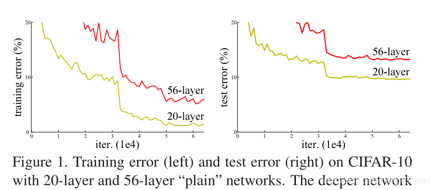
- However, once the number of layers reaches a certain threshold, the accuracy of model training and recognition begins to degrade. This drop in accuracy is not caused by overfitting, as the accuracy for both training and validation data gets worse. Increasing the network depth not only fails to optimize network performance, but instead leads to a decline in output accuracy. This phenomenon is known as the degradation problem of deep networks.
As shown in the figure below, a deeper network (56 layers vs. 20 layers) not only fails to bring better performance, but actually “degrades” on both the training and test sets.
It is worth noting that the problem addressed by ResNet is not the vanishing or exploding gradient problem that occurs during the backpropagation of deep networks. Vanishing and exploding gradients happen because, as network depth increases, gradient values tend to approach zero or remain infinite during the forward-backward pass of training, causing network parameters to fail to update or remain in a divergent state. In fact, these two issues have largely been mitigated by introducing BatchNorm into networks. The “degradation” problem tackled by ResNet is an entirely new issue independent of vanishing/exploding gradients.
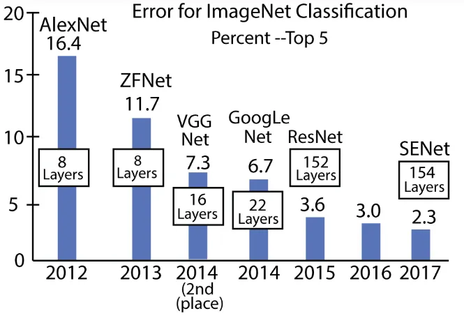
ResNet solved the aforementioned network degradation problem by introducing residual blocks into the model architecture, allowing the depth of deep networks to increase dramatically. As can be seen from the figure below, GoogLeNet, the winner of the 2014 ImageNet dataset image recognition competition, had only 22 layers, whereas ResNet, the winner in 2015, reached a network depth of 152 layers.
Residual Blocks
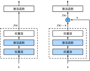
Traditional neural network structures generally connect different convolutional layers, pooling layers, and fully connected layers in a simple sequential order. Each layer in the network only receives information from its immediate predecessor without skipping layers to receive outputs from earlier ones, and each layer’s output is only passed to the immediate next layer. The connection pattern of a normal block on the left side of the figure below illustrates this. With such a sequential pattern, as network depth increases, this single connection method leads to network performance degradation.
In contrast, ResNet introduces the concept of residual blocks. Building upon traditional network connections, shortcut connections are added so that the model’s input data can propagate forward more rapidly through cross-layer connections, as shown on the right side of the figure below.
Why is Residual Mapping Feasible?
Suppose our original input is $x$, and the ideal mapping we expect the network to learn is $f(x)$. If a normal connection structure of traditional neural network patterns is used, the network needs to directly fit the mapping $f(x)$ from the input $x$ of the network block. However, if a residual block pattern is adopted, the block itself does not need to fit $f(x)$; it only needs to fit the residual mapping $f(x) - x$. Learning residual mapping is easier to implement and optimize in reality, which is the underlying logic of how residual blocks solve the problem.
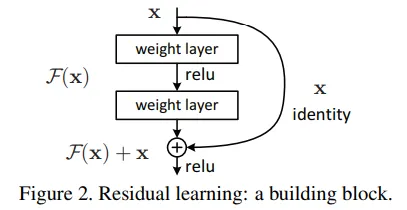
Let’s explain this using the figure below. The mapping that the following network block needs to learn is $H(x)$. If we directly use its input $x$ to learn and train the corresponding mapping $H(x)$, this is what traditional network connections do. For the residual block used in ResNet, the input remains $x$, and the target to be learned is still $H(x)$. By routing the input $x$ directly to the output via a shortcut connection and adding it to the output of the residual block $F(x)$, we get the output of the entire module $H(x)$. In this way, the learning objective for the internal parameters of the residual block is no longer the direct mapping from $x$ to $H(x)$, but rather the mapping from $x$ to $F(x)$ (i.e., $H(x) - x$). Learning and optimizing residuals in a neural network is much easier than directly learning the final mapping.
Let’s take a simple example. Assume the input $x$ is 2.9, and the model’s expected output $H(x)$ is 3.0, with a difference between them of $3.0 - 2.9 = 0.1$.
When using a normal block with a traditional network structure to perform the above mapping, the error variation from input to output is evaluated based on the expected output of 3.0. If the residual block is used to implement this mapping, the training target for the internal parameters of the residual block is the residual $F(x) = H(x) - x = 0.1$. In other words, the training error variation of this network block is evaluated based on this difference of 0.1.
From this, we can find that adopting the residual approach can make the error variations during model training more prominent, making the model easier to train and converge.
Structure of Typical Residual Blocks
In their paper, the authors proposed two residual block structures, as shown in the figure below:
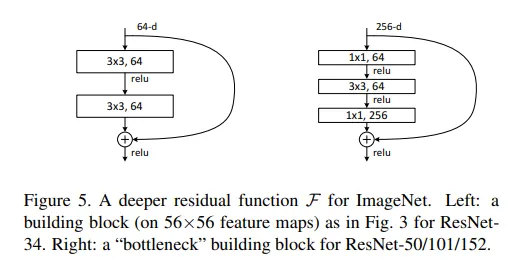
For networks with fewer layers, the basic residual block is constructed using the sequential $3\times3$ convolution - ReLU - $3\times3$ convolution structure shown on the left. For networks deeper than 50 layers, considering training depth and time, the authors proposed the bottleneck design shown on the right. This design introduces a $1\times1$ convolution to reduce dimensions and then another $1\times1$ convolution to restore dimensions. While saving a large number of parameters, it balances the performance and time complexity of deep networks.
ResNet Model Architecture
ResNet has versions with different numbers of network layers, such as 18, 34, 50, 101, and 152 layers. Among them, the most commonly used is the 50-layer network structure, namely ResNet-50.
The overall architecture of the ResNet model can basically be divided into three parts: the input layer, the intermediate sequence of residual blocks, and the final output layer. The input and output layers are identical across all versions of ResNet; the differences among versions lie primarily in the number and structure of the intermediate residual blocks.
The input layer of ResNet—namely the first two layers of its network structure—is identical to that introduced in GoogLeNet from the notes Learning Classical CNN Network Architectures: GoogLeNet: The input image first passes through a $7\times7$ convolution with a stride of 2, outputting feature maps with 64 channels, followed by a $2\times2$ max pooling layer with a stride of 2.
The intermediate residual block section of ResNet consists of consecutively connected basic residual blocks. However, for different versions of ResNet models, the configuration and quantity of residual blocks they contain vary.
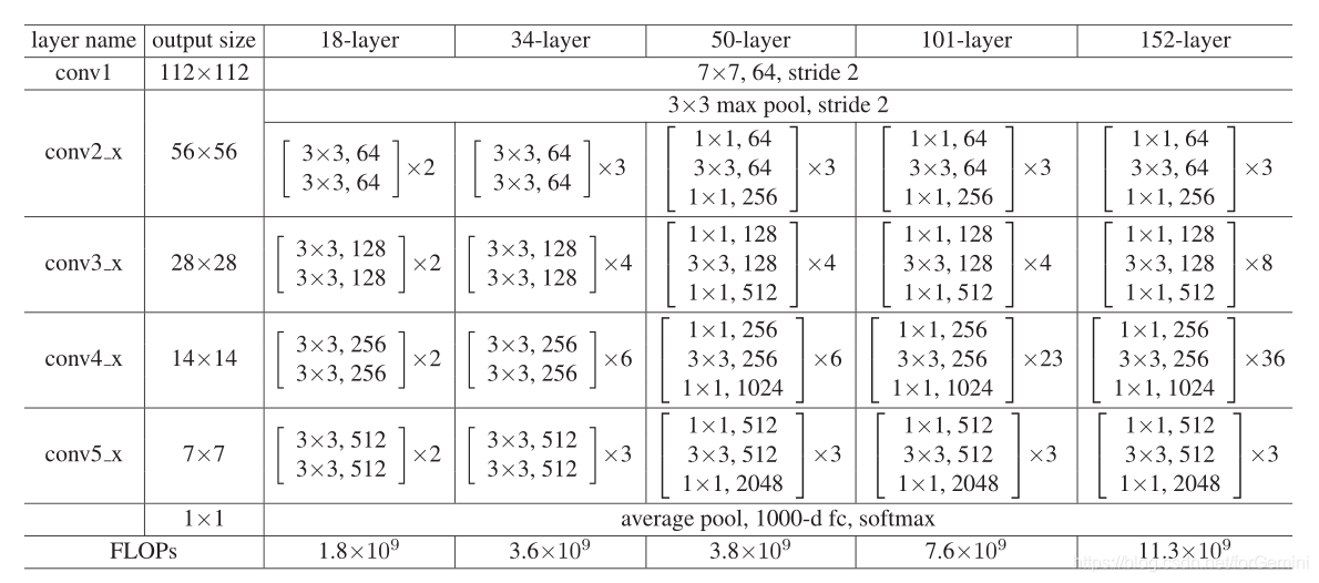
Taking ResNet-34 as an example, the residual block section contains: three consecutive 64-channel $3\times3$ convolutional residual blocks, four consecutive 128-channel $3\times3$ convolutional residual blocks, six consecutive 256-channel $3\times3$ convolutional residual blocks, and three consecutive 512-channel $3\times3$ convolutional residual blocks. Ultimately, it outputs $7\times7\times512$ feature maps to the output layer section. The entire ResNet-34 model structure consists of a total of 1 $7\times7$ convolutional layer, 32 $3\times3$ convolutional layers, and one fully connected layer, totaling 34 parameter layers. The figure below shows the network architecture diagram of the ResNet-34 model:

The feature maps output by the residual block section then pass through a global average pooling layer and are fed into the final fully connected layer with 1,000 neurons. Combined with the Softmax activation function, this achieves the recognition probability output for the 1,000 recognition categories of the ImageNet dataset.