Learning Classical CNN Network Architectures: GoogLeNet

11 Sep, 2025
- AI

This article provides a comprehensive and detailed summary of the problems inherent in traditional convolutional neural networks and the design principles of the classic GoogLeNet architecture in the field of computer vision and image recognition.

Problems in AlexNet and VGGNet

In the previous two notes, Learning Classical CNN Network Architectures: AlexNet and Learning Classical CNN Network Architectures: VGGNet, the architectures and implementations of AlexNet and VGGNet—two classic CNN models—were summarized respectively.

Relatively speaking, AlexNet has fewer layers and parameters, which limits the network’s ability to extract and learn complex patterns from data, resulting in suboptimal ultimate recognition and detection efficiency.

VGGNet increased the depth of the CNN neural network, reaching 16 and 19 parameter layers. However, other issues caused by this increased depth naturally arose:

First is the vanishing gradient problem. As is well known, during the training of neural networks, loss functions are used to evaluate model performance. Based on the loss value, backpropagation combined with gradient descent is used to update parameters layer by layer from the output layer backward, thereby reducing the final loss function output. However, as the network depth increases, the backpropagating gradient signal shrinks progressively as it passes through earlier layers, ultimately making it difficult for parameters in the network (especially those in the earlier layers) to receive effective updates during training.
Second, deep models have excessively high computational demands. Taking the VGG16 network model as an example, its parameters reach up to 138M, and the model size exceeds 500MB, requiring substantial computational power for both training and inference.

The GoogLeNet architecture redesigns traditional CNN network structures to address these issues and has achieved great application success. GoogLeNet, also known as Inception-v1, was first proposed in 2014 and won first place in the 2014 ILSVRC competition, achieving a Top-5 Error of only 6.67%. Even more remarkably, GoogLeNet has only 6.8M parameters—9 times fewer than AlexNet and an impressive 20 times fewer than VGG16.

The biggest innovation of GoogLeNet is the introduction of the Inception module, which is why GoogLeNet is also referred to as InceptionNet.

Inception Module

An Inception module is a building block that allows data to be processed in parallel across multiple scales, enabling the network to capture features at different scales more effectively than previous classic convolutional neural network architectures.

An Inception module typically consists of multiple convolutional layers, each using a different kernel size. Unlike previous network models, the multiple convolutional layers in an Inception module operate in parallel. Thus, for the exact same input feature map, the network can compute using convolutional kernels of various sizes. Once these convolutional layers complete their computations, their outputs are concatenated and passed to a pooling layer for further processing. This is the overarching design philosophy of the Inception module.

From a structural perspective, the Inception modules proposed in GoogLeNet can be classified into two types: the Native type and the Dimensionality Reduction type.

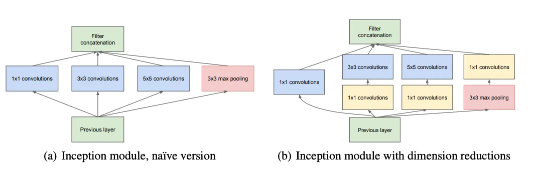
The common characteristic of both Inception module types is that input data obtained from the previous layer’s feature map undergoes parallel processing via 1x1 convolutions, 3x3 convolutions, 5x5 convolutions, and 3x3 max pooling. The outputs from these four paths are concatenated to form the final output of the Inception module. Their difference lies in the fact that: The dimensionality-reduced version of the Inception module adds a 1x1 convolution operation before the 3x3 and 5x5 convolutions, as well as after the 3x3 max pooling.

Among them:

The 1x1 convolutional block is used to capture local details at the pixel level of the feature map while keeping its spatial resolution unchanged.
The 3x3 convolutional block captures mid-range features from the input feature map.
The 5x5 convolutional block is used to capture broader-range features.
The independent 3x3 max pooling block helps preserve salient responses of the original features (such as edges and textures).

As mentioned earlier, the difference between the native module and the dimensionality-reduced module is that the latter incorporates three additional 1x1 convolution operations—placed before the 3x3 and 5x5 convolutions and after the 3x3 max pooling, respectively. The purpose of the two 1x1 convolutions placed before the 3x3 and 5x5 convolutions is to reduce computational complexity and the number of parameters; whereas the 1x1 convolution placed after the 3x3 max pooling is used to control the number of output channels (otherwise, the pooled channel count would match the input channel count, resulting in an excessively large total channel count). Regardless, the output feature maps from all four paths share the same spatial resolution, making it convenient to concatenate them along the depth dimension.

Thus, in the dimensionality-reduced version of the Inception module, the 1x1 convolution in the independent pooling path serves a completely different purpose from the extra 1x1 convolutions added in the convolutional paths.

How 1x1 Convolutions Reduce Computational Cost

In the dimensionality-reduced Inception module, the 1x1 convolutions added before the 3x3 and 5x5 convolutions are primarily intended to reduce the number of parameters and computational cost.

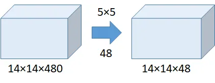
Taking the following figure as an example, without using a 1x1 convolution, converting a feature map from $14 \times 14 \times 480$ to $14 \times 14 \times 48$ using a 5x5 convolution results in a computational cost as high as: $(14 \times 14 \times 480) \times (5 \times 5) \times 48 = 112.9\text{M}$.

When a 1x1 convolutional layer is inserted between the two feature maps, as shown in the figure below, the computational cost drops dramatically:

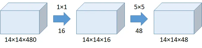
Here, the computational cost of the 1x1 convolution is $(14 \times 14 \times 480) \times (1 \times 1) \times 16 = 1.5\text{M}$, and the computational cost of the 5x5 convolution is $(14 \times 14 \times 16) \times (5 \times 5) \times 48 = 3.8\text{M}$. Combined, they total only 5.3M—a mere 1/20th of the computation without the 1x1 convolution!

How the Inception Module Performs Output Concatenation

As described above, an Inception module processes input data through four independent paths. After processing, the outputs of these four paths are concatenated at the output stage of the Inception module. The primary prerequisite for concatenating the outputs of the four paths is that their feature map resolutions must be identical.

Therefore, the four independent channels are intentionally designed with a stride of 1 and appropriate padding to ensure that the output feature map resolutions match across all channels under the same output data dimensions:

1x1 convolution path: padding=0
3x3 convolution path: padding=1
5x5 convolution path: padding=2
3x3 max pooling path: padding=1

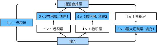
With the above settings, the spatial resolutions of the output feature maps from all four channels remain identical after processing the same input data, while only their channel counts (i.e., the number of feature maps in each channel) differ. When the output feature map resolutions across all four channels are identical, concatenating them becomes straightforward: one simply stacks the feature maps of the four channels side by side along the channel dimension.

Taking the first Inception module (3a) in the GoogLeNet (Inception V1) paper as an example, the input tensor shape from the previous layer is $192 \times 28 \times 28$, produced by preceding convolutional and pooling layers.

Processing occurs across the four paths of the Inception module:

1x1 convolution outputs 64 channels with a $28 \times 28$ resolution ($64 \times 28 \times 28$).
3x3 convolution first reduces dimensions to 96 channels via a 1x1 convolution ($96 \times 28 \times 28$), then outputs 128 channels via a 3x3 convolution with padding=1 ($128 \times 28 \times 28$).
5x5 convolution first reduces dimensions to 16 channels via a 1x1 convolution ($16 \times 28 \times 28$), then outputs 32 channels via a 5x5 convolution with padding=2 ($32 \times 28 \times 28$).
3x3 max pooling first applies 3x3 max pooling (padding=1) maintaining 192 channels ($192 \times 28 \times 28$), then reduces the channel count to 32 via a 1x1 convolution ($32 \times 28 \times 28$).

Finally, concatenating the outputs of these four independent flows yields a total feature map of $64 + 128 + 32 + 32 = 256$ channels with a $28 \times 28$ resolution as the final output of the Inception module.

Global Average Pooling

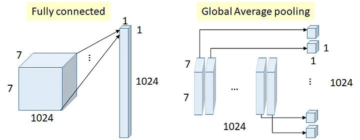
In traditional convolutional neural network architectures, consecutive fully connected layers are used to classify images based on feature data extracted by convolutional layers. The biggest drawback of fully connected layers is their excessive parameter count, leading to severe overfitting. To address this issue, GoogLeNet adopted the same approach as Network in Network (NiN), using global average pooling to replace fully connected layers. This not only solves the problems of excessive parameters and overfitting in traditional models but also noticeably improves classification accuracy, as demonstrated by practical data testing.

The figure below illustrates the different computational logic between a fully connected layer and a global average pooling layer given the same input feature vector. For more details on global average pooling, please refer to Learning Classical CNN Network Architectures: NiN.

Auxiliary Classifier

GoogLeNet has a total of 22 layers. In deep networks, during backpropagation and gradient calculation, gradients diminish progressively across intermediate layers moving backward, ultimately leading to the vanishing gradient problem where parameters in the earlier layers of the network cannot be updated effectively.

GoogLeNet attempts to solve this problem by introducing an Auxiliary Classifier. The core idea is to attach a small classification sub-network (Auxiliary Classifier) to intermediate parts of the network. This sub-network performs classification based on the feature maps from earlier layers and computes its own loss value. During model training, this loss is added to the model’s final output loss to amplify gradient signals and mitigate the vanishing gradient effect.

Auxiliary classifiers are used exclusively during the training phase; during inference, only the main network output is retained, meaning inference speed remains unaffected.

In the GoogLeNet architecture, an Auxiliary Classifier is added after the 4a and 4d Inception modules, respectively (refer to the overall GoogLeNet network structure section below). The structure of each Auxiliary Classifier is as follows:

The input consists of the feature maps output by the respective Inception module, such as feature maps with 512 channels and a $14 \times 14$ resolution.
5x5 average pooling: Applies a 5x5 average pooling operation with a stride of 3 to the input feature maps, resulting in 512 channels with a $4 \times 4$ resolution.
1x1 convolution: Reduces the channel count from 512 to 128 using a 1x1 convolution, outputting 128 channels at a $4 \times 4$ resolution.
Flattens the feature map and connects it to a fully connected layer with 1024 neurons using the ReLU activation function.
Adds a Dropout operation with a dropout rate of 0.7.
Connects to a fully connected layer with 1000 neurons, corresponding to the 1000 categories of the ImageNet dataset.
The 1000-neuron multiply-accumulate output passes through a softmax operation to yield a 1000-dimensional prediction vector.

The prediction output of the Auxiliary Classifier is compared against the ground truth labels to compute the auxiliary loss. The loss values generated by the two auxiliary classifiers are multiplied by a weight of 0.3 and added to the main network’s classification loss to form the total network loss:

$$ TotalLoss=Loss_{main}+0.3Loss_{4a}+0.3Loss_{4d} $$

During network parameter training, this TotalLoss is backpropagated to update the network parameters.

Overall Structure of GoogLeNet

With the background information above, understanding the overall architecture of GoogLeNet becomes relatively straightforward:

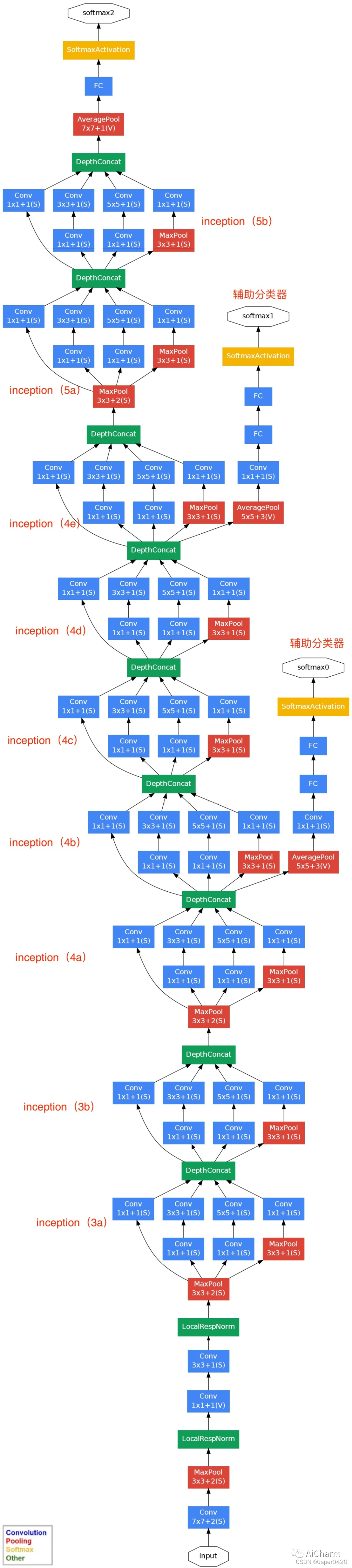
From the overall architecture, we can observe:

The beginning of GoogLeNet reduces the input image resolution through sequential convolutional and pooling operations.
It then continuously extracts image features through 9 Inception modules, grouped into 3 stages ($2 + 5 + 2$). Consecutive modules within each Inception stage are directly connected, while stages are bridged by 3x3 max pooling layers.
The output of the final Inception module passes through global average pooling followed by a fully connected layer to perform final image classification.
Additionally, Auxiliary Classifiers are attached to the outputs of Inception 4a and 4d to provide stage-specific losses that assist the training process.

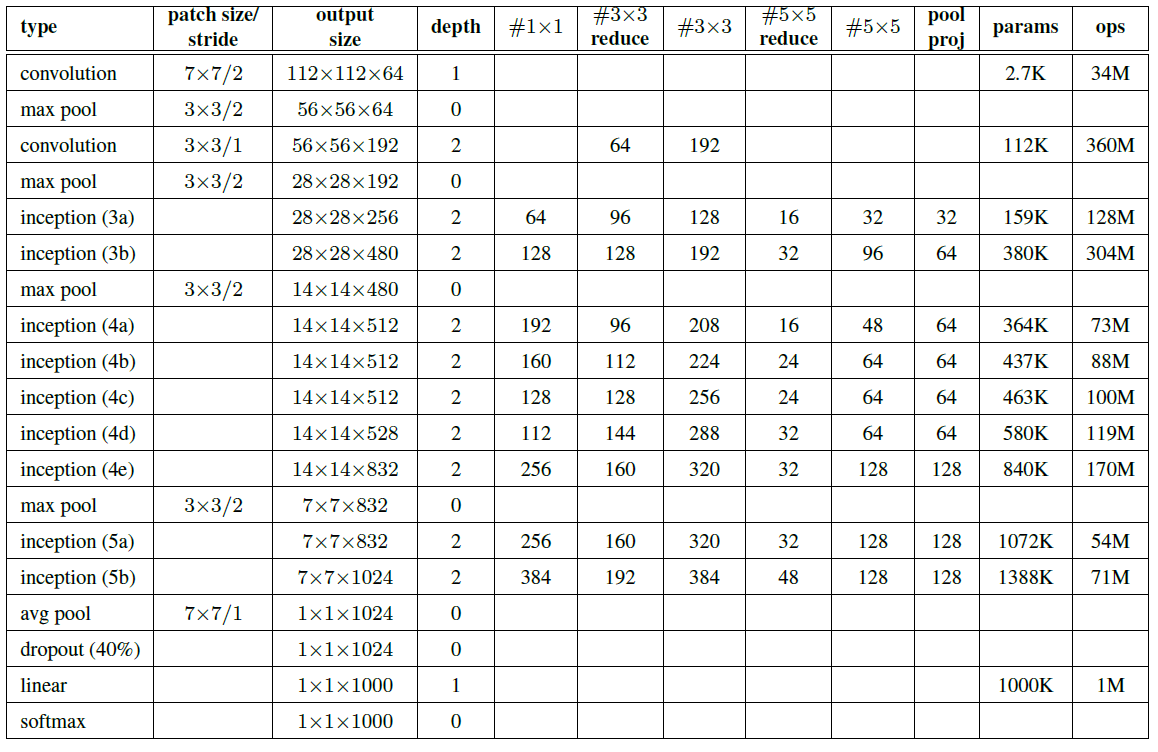
The data dimensions and parameter counts for each layer in GoogLeNet are detailed in the table below:

References

#CNN