Learning Classical CNN Model Architectures: NiN
- 10 Sep, 2025
This article summarizes the design philosophy, overall architecture, and specific implementation details of NiN (Network in Network), a classic model in convolutional neural networks.
The design patterns of the three classical convolutional neural network models—LeNet, AlexNet, and VGGNet—are largely identical: they perform feature extraction through a series of convolutional and pooling layer combinations, flatten the extracted feature data, and then feed it into a series of fully connected layers for classification to ultimately output image recognition probabilities.
The aforementioned classical convolutional neural network design paradigm presents two major design challenges:
- The fully connected layers responsible for image classification based on feature data contain an excessive number of parameters. For instance, in the VGG16 network, the parameter count reaches up to 138MB, and the storage space occupied by the model parameters exceeds 500MB.
- It is impractical to add fully connected layers in the first half of the network to increase non-linearity; doing so would disrupt spatial structures while demanding even more parameters and memory.
To address these two architectural design issues, Network in Network (NiN), published in 2013 by Min Lin from the National University of Singapore, introduced a novel design perspective to the architectural philosophy of classical convolutional neural networks.
The two most significant innovations of the NiN architecture over traditional CNNs are the MLP convolutional layer and the global average pooling layer.
MLP Convolutional Layers
The convolutional calculation logic of traditional convolutional layers has already been described in detail in the article Detailed Explanation of Convolution and Pooling Calculations in Convolutional Neural Networks and will not be repeated here. It is illustrated simply via a convolutional calculation animation:
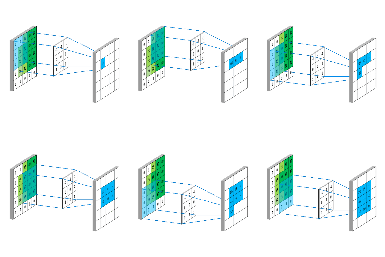
In summary, the traditional convolutional layer calculation formula is shown in the figure below, where $(i,j)$ is the index of the pixel position in the input feature map, $x_{i,j}$ represents the pixel at the corresponding position, and $W$ represents the parameters of the convolution kernel. Thus, convolution calculation is essentially the multiply-accumulate result of the pixels at and surrounding $(i,j)$ with the corresponding weights of the convolution kernel, which is then processed through the ReLU activation function to yield the feature map of the convolution.

In the implementation of the NiN network, convolution calculations are organized in the manner of an MLP Block. A typical structure of an MLP Block is shown in the figure below:
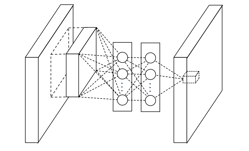
For each MLP Block, the input is either the original 3-channel RGB image or multiple feature maps output by the previous MLP Block. Inside each MLP Block, there are three consecutive convolutional layers, where the input to each layer is the output of the preceding one. The convolution calculation of the first convolutional layer is identical to standard convolution, whereas the subsequent two layers are $1\times1$ convolutional layers. The $1\times1$ convolution still calculates the multiply-accumulate of feature map pixel values and weights, followed by non-linear processing using the ReLU activation function.
The following code explains the structure and calculation logic of each MLP Block:
def nin_block(out_channels, kernel_size, strides, padding):
    return nn.Sequential(
        nn.LazyConv2d(out_channels, kernel_size, strides, padding), nn.ReLU(),
        nn.LazyConv2d(out_channels, kernel_size=1), nn.ReLU(),
        nn.LazyConv2d(out_channels, kernel_size=1), nn.ReLU())
Each MLP Block contains 3 convolutional layers: a standard convolutional layer + ReLU activation, followed by two consecutive $1\times1$ convolutional layers + ReLU activation. In terms of network architecture, each MLP Block is generally followed by a max-pooling layer.
Global Average Pooling Layer
In traditional convolutional neural network architectures, multiple fully connected layers are generally used to implement feature classification. The approach involves flattening the feature map produced by the last convolutional layer into a 1D vector, passing it through a succession of fully connected layers, and finally using a softmax layer for logistic regression classification. The primary issues with this approach are: an excessive number of parameters in the fully connected layers, and overfitting caused by multiple fully connected layers.
The NiN network replaces fully connected layers with global average pooling operations in an attempt to resolve the issues of excessive parameters and overfitting in the latter half of classical convolutional neural networks. The specific procedure of global average pooling is to make the number of output feature maps from the final convolutional layer equal to the number of classification categories (e.g., 1000 for the ImageNet dataset, or 10 for the MNIST dataset). Then, the average value of each feature map is taken to output a vector, upon which a softmax operation is applied (for the calculation workflow of the softmax operation, refer to Detailed Summary of Softmax Classifier Calculation Workflow), ultimately outputting the recognition probabilities for each category.
The workflow of the global average pooling operation is illustrated in the figure below:
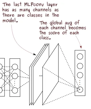
Taking the ImageNet dataset (which has 1000 image classification categories) as an example, the global average pooling layer obtains 1000 feature maps from its preceding MLP convolutional layer. During global average pooling, an average calculation is performed on each feature map to obtain its mean value, ultimately yielding a vector composed of 1000 mean values. A softmax operation is then executed on this vector to output the recognition probability for each category.
As can be seen, the calculation logic of the global average pooling layer above is similar to that of ordinary average pooling and thus requires absolutely no parameters. This drastically reduces the number of model parameters (in reality, the majority of parameters in classical CNNs stem from fully connected layers) and avoids the overfitting problems inherent to traditional fully connected layers.
Summary of NiN Network Architecture
The overall structure of the NiN network is shown in the figure below. The image input is still a $224\times224$ resolution RGB 3-channel image. After convolutional processing through four consecutive MLP Blocks, the final MLP Block outputs 1000 feature maps of size $6\times6$. These feature maps are passed through the average calculation of the global average pooling layer and softmax activation to output recognition probabilities for 1000 categories.
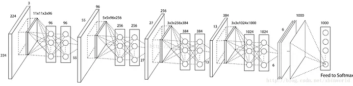
You can refer to the figure below to understand the feature map dimensions and calculation types of each layer in the NiN architecture diagram above. Although the NiN network appears to have considerably more layers than the VGG network, its parameter count is much smaller than VGG’s due to the omission of fully connected layers.
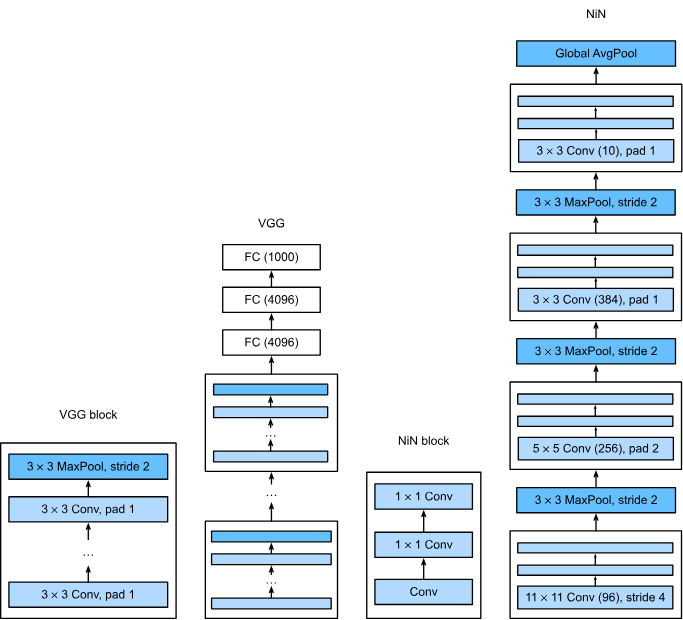
The complete implementation code for the NiN network, based on the nin_block structure defined above, is as follows:
class NiN(d2l.Classifier):
    def __init__(self, lr=0.1, num_classes=10):
        super().__init__()
        self.save_hyperparameters()
        self.net = nn.Sequential(
            nin_block(96, kernel_size=11, strides=4, padding=0),
            nn.MaxPool2d(3, stride=2),
            nin_block(256, kernel_size=5, strides=1, padding=2),
            nn.MaxPool2d(3, stride=2),
            nin_block(384, kernel_size=3, strides=1, padding=1),
            nn.MaxPool2d(3, stride=2),
            nn.Dropout(0.5),
            nin_block(num_classes, kernel_size=3, strides=1, padding=1),
            nn.AdaptiveAvgPool2d((1, 1)),
            nn.Flatten())
        self.net.apply(d2l.init_cnn)