Learning CNN Classical Network Architectures: VGGNet
- 09 Sep, 2025
This article provides a detailed summary of the architecture of the classic VGGNet model in the field of computer vision and image recognition, along with its implementation in PyTorch.
Introduction to VGGNet Architecture
VGG stands for Visual Geometry Group. The original design concept of VGGNet was to improve model performance by increasing the depth of the convolutional neural network. VGGNet secured second place in the 2024 ImageNet Large Scale Visual Recognition Challenge (ILSVRC) (GoogLeNet took first place that year), achieving a top-5 accuracy (whether the ground truth label is among the top 5 highest probability predictions from the model) of 92.7%. In many subsequent models, VGGNet’s network structure is often used as a backbone for image feature extraction.
Typical models in the VGGNet architecture family include VGG16, VGG19, and VGG34, where the numbers indicate the count of parameter layers (i.e., convolutional layers and fully connected layers) contained in each model architecture.
The following figure illustrates the network architecture of VGG16:
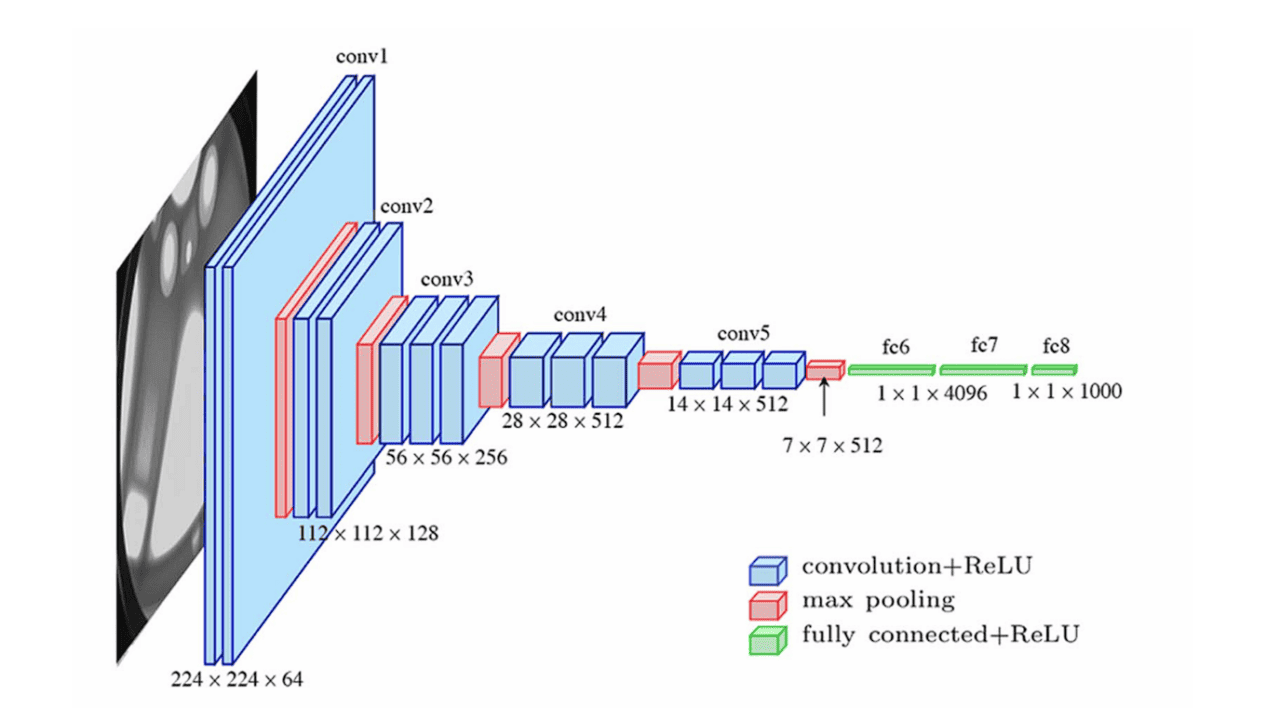
- Throughout the entire VGG16 network architecture, it contains 13 convolutional layers, 5 pooling layers, and 3 fully connected layers, totaling 16 parameter layers (convolutional and fully connected layers combined).
- The model takes an RGB 3-channel image with a resolution of 224x224 as input and outputs predicted probabilities for 1000 image classification categories (since VGG16 was designed to predict the ImageNet dataset, which has 1000 classes).
- From a structural design standpoint, it remains a standard convolutional neural network. The entire architecture is divided into two parts: the first half is the image feature extraction component composed of convolutional and pooling layers, while the second half is the image classification component composed of fully connected layers. Therefore, the network structure has no fundamental difference from LeNet and AlexNet as summarized in Learning CNN Classical Network Architectures: LeNet and Learning CNN Classical Network Architectures: AlexNet, except that it is much deeper. Because of this significantly increased depth compared to LeNet and AlexNet, the number of parameters in VGG16 reaches 138M.
Compared to VGG16, VGG19 has 3 additional convolutional layers—specifically, one extra convolutional layer in each of the conv3, conv4, and conv5 blocks—while all other parts (including kernel sizes, channel counts, pooling strategies, and fully connected layer structures) remain completely identical.
In the original VGGNet paper, the authors provided a total of 6 network configurations, labeled A through E. VGG16 corresponds to configuration D, while VGG19 corresponds to configuration E.
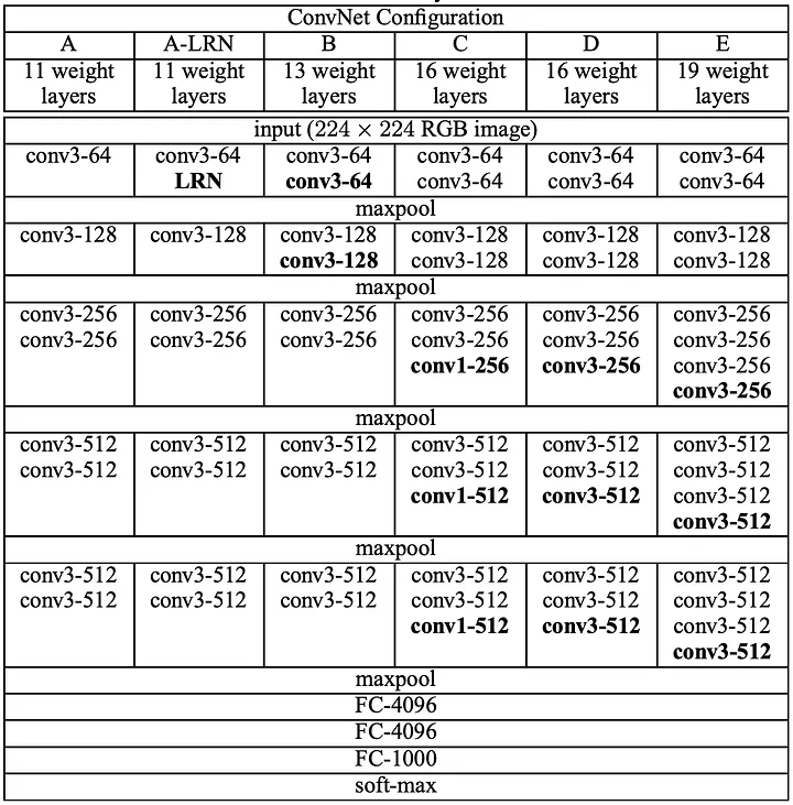
As seen in the table above, the network architectures of the 6 configurations (A-E) are largely similar, with the only differences lying in the number of convolutional layers in each block.
Parameter Configuration of VGG16 Network Layers
The following figure shows the hyperparameter settings for each layer in the VGG16 network architecture:
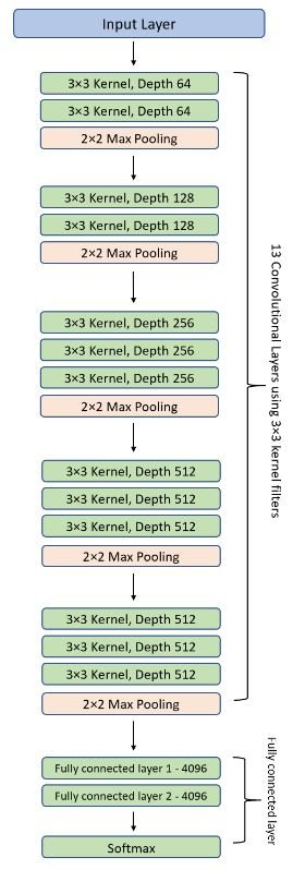
- As shown, the number of convolutional filters in the conv1, conv2, conv3, and conv4/conv5 sections of the VGG16 network structure is 64, 128, 256, and 512, respectively. The number of filters doubles in each successive convolutional block, which is a crucial design principle of the VGG16 architecture.
- The kernel size for all convolutional layers is 3x3 (in sharp contrast to the larger filter sizes used in AlexNet), and the convolution stride is uniformly set to 1. All pooling layers are 2x2 max pooling with a stride of 2.
- Regarding activation functions, except for the final output layer which uses the multi-class softmax activation function, all other convolutional and fully connected layers use ReLU.
- For the final three fully connected layers, the first two layers both contain 4096 neurons, and the final output layer corresponds to the 1000 categories of the ImageNet dataset, containing 1000 neurons.
PyTorch Implementation of VGGNet
The PyTorch code implementation of the VGG16 network structure is shown below:
class VGG16(nn.Module):
    def __init__(self, num_classes=1000):
        super(VGG16, self).__init__()

        # Convolutional layers - 5 convolutional blocks
        # Conv Block 1: 2 conv layers, 64 output channels
        self.conv1_1 = nn.Conv2d(in_channels=3, out_channels=64, kernel_size=3, padding=1)
        self.conv1_2 = nn.Conv2d(in_channels=64, out_channels=64, kernel_size=3, padding=1)
        # Conv Block 2: 2 conv layers, 128 output channels
        self.conv2_1 = nn.Conv2d(in_channels=64, out_channels=128, kernel_size=3, padding=1)
        self.conv2_2 = nn.Conv2d(in_channels=128, out_channels=128, kernel_size=3, padding=1)
        # Conv Block 3: 3 conv layers, 256 output channels
        self.conv3_1 = nn.Conv2d(in_channels=128, out_channels=256, kernel_size=3, padding=1)
        self.conv3_2 = nn.Conv2d(in_channels=256, out_channels=256, kernel_size=3, padding=1)
        self.conv3_3 = nn.Conv2d(in_channels=256, out_channels=256, kernel_size=3, padding=1)
        # Conv Block 4: 3 conv layers, 512 output channels
        self.conv4_1 = nn.Conv2d(in_channels=256, out_channels=512, kernel_size=3, padding=1)
        self.conv4_2 = nn.Conv2d(in_channels=512, out_channels=512, kernel_size=3, padding=1)
        self.conv4_3 = nn.Conv2d(in_channels=512, out_channels=512, kernel_size=3, padding=1)
        # Conv Block 5: 3 conv layers, 512 output channels
        self.conv5_1 = nn.Conv2d(in_channels=512, out_channels=512, kernel_size=3, padding=1)
        self.conv5_2 = nn.Conv2d(in_channels=512, out_channels=512, kernel_size=3, padding=1)
        self.conv5_3 = nn.Conv2d(in_channels=512, out_channels=512, kernel_size=3, padding=1)

        # Pooling layer
        self.pool = nn.MaxPool2d(kernel_size=2, stride=2)

        # Dropout layers
        self.dropout1 = nn.Dropout(p=0.5)
        self.dropout2 = nn.Dropout(p=0.5)

        # Fully connected layers
        self.fc1 = nn.Linear(in_features=512*7*7, out_features=4096)
        self.fc2 = nn.Linear(in_features=4096, out_features=4096)
        self.fc3 = nn.Linear(in_features=4096, out_features=num_classes)

    def forward(self, x):
        # Conv Block 1
        x = F.relu(self.conv1_1(x))
        x = F.relu(self.conv1_2(x))
        x = self.pool(x)

        # Conv Block 2
        x = F.relu(self.conv2_1(x))
        x = F.relu(self.conv2_2(x))
        x = self.pool(x)

        # Conv Block 3
        x = F.relu(self.conv3_1(x))
        x = F.relu(self.conv3_2(x))
        x = F.relu(self.conv3_3(x))
        x = self.pool(x)

        # Conv Block 4
        x = F.relu(self.conv4_1(x))
        x = F.relu(self.conv4_2(x))
        x = F.relu(self.conv4_3(x))
        x = self.pool(x)

        # Conv Block 5
        x = F.relu(self.conv5_1(x))
        x = F.relu(self.conv5_2(x))
        x = F.relu(self.conv5_3(x))
        x = self.pool(x)

        # Flatten operation
        x = x.view(-1, 512*7*7)

        # Fully connected layers
        x = F.relu(self.fc1(x))
        x = self.dropout1(x)
        x = F.relu(self.fc2(x))
        x = self.dropout2(x)
        x = self.fc3(x)

        return x