Learning Classical CNN Network Architectures: AlexNet
- 04 Sep, 2025
This article provides a detailed summary of the architecture of the classic AlexNet model in the field of computer vision and image recognition, along with its implementation in PyTorch.
In the previous article, Learning Classical CNN Network Architectures: LeNet, we explored Yann LeCun’s LeNet-5 network model designed for handwritten digit recognition. Continuing our study of classic model frameworks in computer vision, this article summarizes AlexNet, which stood out and won the ImageNet Large Scale Visual Recognition Challenge.
Brief History of AlexNet
In the 2012 ImageNet Large Scale Visual Recognition Challenge (ILSVRC), AlexNet—proposed by Alex Krizhevsky, Ilya Sutskever, and Geoffrey E. Hinton—won the championship. On the competition’s most crucial Top-5 Error Rate metric, AlexNet achieved a landslide victory, outperforming the runner-up by a remarkable 10 percentage points:
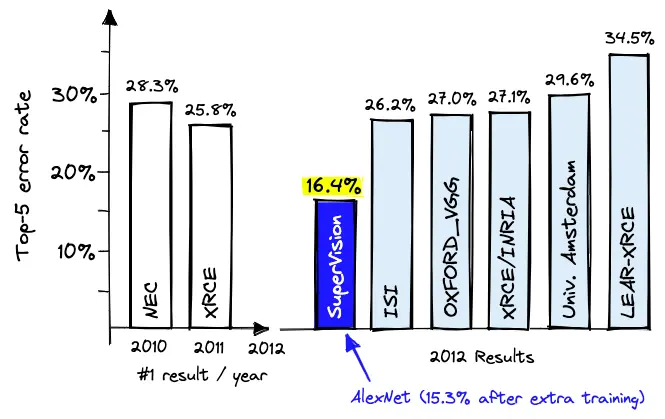
It was precisely because of AlexNet’s exceptional performance in this competition that it sparked a research boom in deep learning within the field of artificial intelligence and computer vision.
AlexNet Network Architecture
The network architecture diagram of AlexNet is shown below:
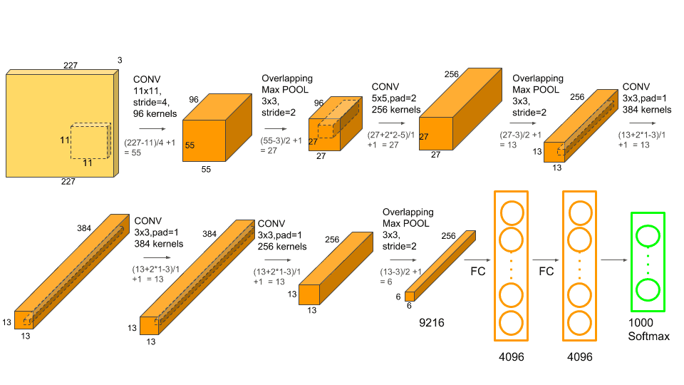
As seen in the figure above, the overall structure of AlexNet is very similar to the LeNet-5 network architecture described in Learning Classical CNN Network Architectures: LeNet. Overall, it can be divided into two parts:
- Image Feature Extraction Section: Consisting of layers from the input layer up to the final max-pooling layer, this part outputs a 6x6x256 dimensional image feature vector.
- Classification Section: Consisting of the final three fully connected layers.
The input to the AlexNet network is an RGB three-channel image with a resolution of 227x227, and the output consists of 1,000 classification probabilities generated via the SoftMax activation function across 1,000 neurons in the output layer. The reason for 1,000 categories is primarily because AlexNet was originally designed to participate in the ImageNet image recognition competition, which contains 1,000 image categories.
The overall network structure of AlexNet contains a total of five convolutional layers, three max-pooling layers, and three fully connected layers.
- The input data consists of RGB three-channel color image data with a 227x227 resolution.
- The first convolutional layer contains 96 kernels of size 11x11x3, with a stride of 4 and the ReLU activation function, ultimately producing 96 feature maps of 55x55 resolution.
- The first pooling layer uses 3x3 max pooling with a stride of 2, outputting 96 feature maps of 27x27 resolution.
- The second convolutional layer contains 256 kernels of size 5x5x96, with a stride of 1, padding of 2, and the ReLU activation function, ultimately producing 256 feature maps of 27x27 resolution.
- The second pooling layer uses 3x3 max pooling with a stride of 2, outputting 256 feature maps of 13x13 resolution.
- The third convolutional layer contains 384 kernels of size 3x3x256, with a stride of 1, padding of 1, and the ReLU activation function, ultimately producing 384 feature maps of 13x13 resolution.
- The fourth convolutional layer contains 384 kernels of size 3x3x384, with a stride of 1, padding of 1, and the ReLU activation function, ultimately producing 384 feature maps of 13x13 resolution.
- The fifth convolutional layer contains 256 kernels of size 3x3x384, with a stride of 1, padding of 1, and the ReLU activation function, ultimately producing 256 feature maps of 13x13 resolution.
- The third pooling layer uses 3x3 max pooling with a stride of 2, outputting 256 feature maps of 6x6 resolution.
- This concludes the feature extraction section of AlexNet. The final pooling layer flattens the output into a 1D vector of 6x6x256 elements, which serves as the input to the first fully connected layer of the classification network.
- The first fully connected layer has 6x6x256 = 9,216 inputs, 4,096 neuron outputs, and uses the ReLU activation function.
- The second fully connected layer accepts 4,096 inputs, has 4,096 neuron outputs, and uses the ReLU activation function.
- The final fully connected layer has 1,000 neuron outputs, corresponding to the 1,000 recognition categories of the ImageNet dataset.
The total number of parameters across the entire network reaches 60 million, primarily concentrated in the final three fully connected layers: $9216 \times 4096 + 4096 \times 4096 + 4096 \times 1000 = 59,621,952$. As we can see, the last three fully connected layers account for the vast majority of all parameters.
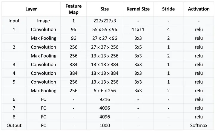
The data dimensions of each layer throughout the network structure are summarized below:
Implementation of AlexNet’s Dual-GPU Architecture
Additionally, in some reference materials, the architecture diagram of AlexNet appears as shown below:
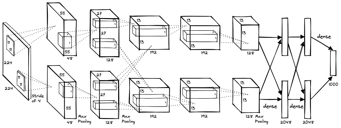
As can be seen, the above architecture diagram divides the entire network into identical upper and lower halves. The input image is fed into both upper and lower sub-networks simultaneously, and they finally merge at the output layer. This architecture diagram actually reflects the original implementation of AlexNet. Because the GPU configuration and processing power at that time were relatively low, training AlexNet on the ImageNet dataset using a single GPU would have been extremely slow. Therefore, Alex split the network into upper and lower parts, with the two sub-networks running in parallel on two graphics cards and merging their output results at the end. This approach significantly accelerated training and inference speeds.
However, regardless of this, from the perspective of network layers and structural design essence, the dual sub-network structure described above is identical to the standard network structure of AlexNet.
Summary of AlexNet’s Key Features
Activation Function
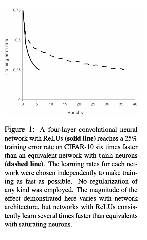
In the network architecture design of AlexNet, the activation function was changed from Sigmoid (used in LeNet-5) to ReLU. This modification helps solve the vanishing gradient problem inherent in Sigmoid activation functions when neural networks become too deep or gradients are too small. At the same time, compared to activation functions like Sigmoid and Tanh, ReLU offers advantages such as faster convergence speed, higher training efficiency, and simpler computation.
The following figure, demonstrated in the AlexNet paper on the CIFAR-10 dataset, highlights the massive advantage of ReLU over the Tanh activation function in terms of training convergence speed:
Max Pooling
Another distinct difference between AlexNet and LeNet-5 is the use of max pooling layers instead of the average pooling layers used in LeNet-5.
The 3x3 max pooling layer with stride=2 adopted by AlexNet is better at retaining important features compared to LeNet-5’s 2x2 average pooling. Furthermore, because $\text{stride} < \text{size}$ ($2 < 3$), the pooling operations overlap, allowing features to be scanned repeatedly and preventing important features from being discarded.
Solutions to Overfitting
The AlexNet paper mentions several countermeasures to address and optimize model training overfitting. Overfitting refers to a scenario where a model and its trained parameters perform exceptionally well on the training dataset, but poorly on new validation and test datasets.
For example, in the implementation of the first two fully connected layers, a dropout=0.5 operation was introduced. During the training process, 50% of the neuron parameters in these two layers are randomly excluded from the forward inference and backward gradient update processes in each training step, thereby improving the generalization capability of the model and its parameters.
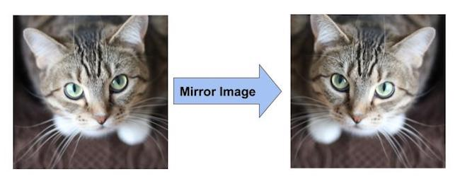
Another example is Data Augmentation. To improve training efficiency, increasing the training dataset is an effective approach. Simply put, Data Augmentation generates new training data by applying various transformations to the existing training image set (i.e., the ImageNet dataset), rapidly increasing the number of training samples at a low cost. Data augmentation methods here include horizontal image flipping, Gaussian noise, and variations in image color and lighting (PCA).
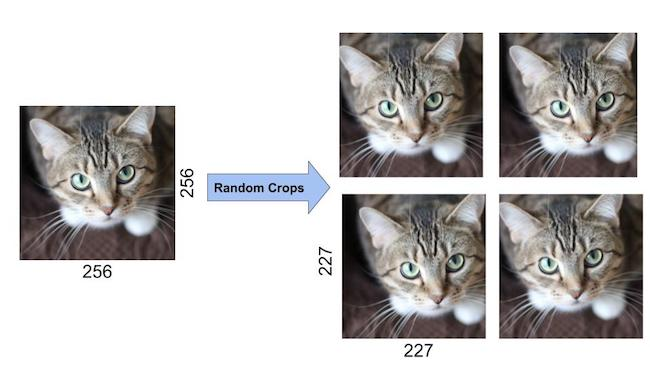
Another technique is random cropping of input images. The image sizes in the ImageNet dataset are not uniform. During AlexNet training, the shorter side of the input image is first resized to 256 pixels, and then the longer side is extended by 128 pixels from the center of the image to the left and right, with excess parts cropped out, resulting in a 256x256 resolution image as training input. As mentioned earlier, the input image resolution of the AlexNet network is 227x227. Therefore, based on this 256x256 resolution input, it is randomly cropped to a 227x227 resolution during each training iteration. This approach significantly multiplies the number of training images (by a factor of 2,048).
Multi-GPU Training
As described in the model structure section above, to accelerate model training and inference execution, the designers of AlexNet split the entire network into two identical sub-networks, utilizing two GTX 580 GPUs running simultaneously to speed up the training process. Because the GTX 580 had only 3GB of VRAM and could not handle heavy computations on its own, splitting the neural network into two independent sub-networks running on separate graphics cards greatly accelerated the training speed.
PyTorch Implementation of AlexNet
The code implementation of AlexNet based on the PyTorch framework is shown below:
class AlexNet(nn.Module):
    def __init__(self, num_classes):
        super(AlexNet, self).__init__()
        self.conv1 = nn.Conv2d(in_channels=3, out_channels=96, kernel_size=11, padding=2, stride=4)
        self.conv2 = nn.Conv2d(in_channels=96, out_channels=256, kernel_size=5, padding=2)
        self.conv3 = nn.Conv2d(in_channels=256, out_channels=384, kernel_size=3, padding=1)
        self.conv4 = nn.Conv2d(in_channels=384, out_channels=384, kernel_size=3, padding=1)
        self.conv5 = nn.Conv2d(in_channels=384, out_channels=256, kernel_size=3, padding=1)

        self.fc1 = nn.Linear(in_features=256*6*6, out_features=4096)
        self.fc2 = nn.Linear(in_features=4096, out_features=4096)
        self.fc3 = nn.Linear(in_features=4096, out_features=num_classes)

    def forward(self, x):
        x = F.relu(self.conv1(x))
        x = F.max_pool2d(x, kernel_size=3, stride=2)
        x = F.relu(self.conv2(x))
        x = F.max_pool2d(x, kernel_size=3, stride=2)
        x = F.relu(self.conv3(x))
        x = F.relu(self.conv4(x))
        x = F.relu(self.conv5(x))
        x = F.max_pool2d(x, kernel_size=3, stride=2)
        x = x.view(-1, 256*6*6)
        x = F.relu(self.fc1(x))
        x = F.relu(self.fc2(x))
        x = self.fc3(x)
        return x
The network architecture exported via Netron.app is illustrated below:
