CNN Classical Network Model Architecture Learning: LeNet

Using LeNet for handwritten digit recognition as an example, this article analyzes the network structure and the overall architecture of a typical Convolutional Neural Network (CNN), establishing a foundational understanding of CNNs used for image recognition and processing.

In the article Introduction to CNN Network Architecture Analysis, we briefly summarized the structure and components of a typical convolutional neural network. In this article, we will use a very classic network—LeNet-5, designed for handwritten digit recognition—to explain the structure and execution flow of CNNs in greater detail.

Introduction to LeNet

LeNet is one of the earliest published convolutional neural networks and also the one with the simplest architecture. It is exceptionally well-suited as an introductory network structure to build a foundational understanding of CNN architecture design and execution flow.

The LeNet model was first proposed in 1989 by Yann LeCun, a researcher at Bell Labs, and was continuously optimized. Its design and application were intended for recognizing handwritten digits (i.e., training and recognition on the well-known MNIST dataset). LeNet was widely used in the United States postal service and automated teller machines (ATMs) to help recognize and process handwritten zip codes and numbers on checks. To this day, some ATMs are still running code written by Yann LeCun and his colleague Leon Bottou in the 1990s!

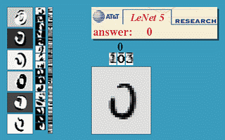
Official LeNet website: MNIST Demos on Yann LeCun’s website

Explanation of LeNet’s Network Architecture

The diagram below illustrates the network architecture of LeNet:

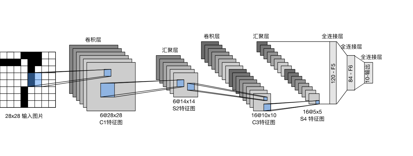
Overall, like all convolutional neural networks, the above network architecture consists of two main parts:

• Feature Extraction Layer: Contains a combination of two convolutional layers + pooling layers (referred to as pooling layers in the diagram above).
• Classification Layer: Contains three fully connected layers.

The basic unit within each convolutional block is a convolutional layer, a sigmoid activation function, and an average pooling layer. The output of the final pooling layer in the feature extraction layer is a 16-channel 5x5 feature map. This feature map is flattened into a 1D vector of 16x5x5 elements, which is then fed into the fully connected layers to perform the classification task. The final fully connected layer has 10 neurons, corresponding to the recognition probabilities for the 10 digits from 0 to 9.

Detailed information on the layer structures and parameter counts of the LeNet network is summarized as follows:

• The input data is a grayscale image with a resolution of 28x28, which is essentially a 28x28 2D array with only a single grayscale channel.
• Convolutional layer C1 contains six 5x5x1 convolution kernels with a padding of 2, so the output of this convolutional layer consists of six 28x28 resolution feature maps. The activation function for the convolution calculation results is Sigmoid.
  • The number of parameters in this layer consists of the weights and biases of the six 5x5x1 convolution kernels, which is 6 x (5 x 5 x 1 + 1).
• Pooling layer S2 uses a 2x2 average pooling operation on the 6-channel 28x28 resolution feature maps from convolutional layer C1, outputting 6-channel 14x14 resolution pooled feature maps.
• Convolutional layer C3 contains sixteen 5x5x6 volumetric convolution kernels with a padding of 0, so the output of convolutional layer C3 consists of sixteen 10x10 resolution feature maps. The activation function for the convolution calculation results is also Sigmoid.
  • The number of parameters in this layer consists of the weights and biases of the sixteen 5x5x6 convolution kernels, which is 16 x (5 x 5 x 6 + 1).
• Pooling layer S4 still uses a 2x2 average pooling operation on the 16-channel 10x10 resolution feature maps from convolutional layer C3, outputting 16-channel 5x5 resolution pooled feature maps.
• The input to the first fully connected layer F5 is the 1D flattened vector of the feature maps output by pooling layer S4. Thus, the input data is a 1D vector of 5x5x16. F5 has 120 neurons, and the activation function is still Sigmoid.
  • The number of parameters in this layer consists of the input weights and biases for the 120 neurons, which is 120 x (5 x 5 x 16 + 1).
• The input to the second fully connected layer F6 comes from the outputs of the 120 neurons in F5. F6 has 84 neurons, and the activation function is Sigmoid.
  • The number of parameters in this layer consists of the input weights and biases for the 84 neurons, which is 84 x (120 + 1).
• The final output layer has 10 neurons, where the output of each neuron corresponds to the recognition probability of a digit from 0 to 9.
  • The number of parameters in this layer consists ofynn the input weights and biases for the 10 neurons, which is 10 x (84 + 1).

Below is a summary of the dimensions of the output vectors at each layer of LeNet during the forward computation process:

Input shape:     torch.Size([1, 1, 28, 28])
Conv1 output shape:      torch.Size([1, 6, 28, 28])
Sigmoid1 output shape:   torch.Size([1, 6, 28, 28])
AvgPool1 output shape:   torch.Size([1, 6, 14, 14])
Conv2 output shape:      torch.Size([1, 16, 10, 10])
Sigmoid2 output shape:   torch.Size([1, 16, 10, 10])
AvgPool2 output shape:   torch.Size([1, 16, 5, 5])
Flatten output shape:    torch.Size([1, 400])
Fc1 output shape:        torch.Size([1, 120])
Sigmoid3 output shape:   torch.Size([1, 120])
Fc2 output shape:        torch.Size([1, 84])
Sigmoid4 output shape:   torch.Size([1, 84])
Fc3 output shape:        torch.Size([1, 10])

Regarding the network structure of LeNet above, note the following:

• In the network structure diagram above, there are a total of 7 layers: two convolutional layers, two pooling layers, and three fully connected layers. However, LeNet in the general sense typically refers to LeNet-5, where the number 5 represents the number of layers containing parameters in the entire network (i.e., two convolutional layers + three fully connected layers).
• In practical CNN implementations, using the ReLU activation function for convolutional layers and max pooling for pooling layers yields better performance. However, neither ReLU nor max pooling existed in the 1980s and 1990s. Therefore, in the original LeNet-5 architecture, the classic Sigmoid activation function was used for convolutional layers, and average pooling was used for pooling layers.

PyTorch Implementation of LeNet

Based on the network architecture of the LeNet-5 model introduced above, the implementation code for this network under the PyTorch framework is as follows:

import torch
import torch.nn as nn
import torch.nn.functional as F

class LeNet(nn.Module):
    def __init__(self):
        super(LeNet, self).__init__()
        self.conv1 = nn.Conv2d(in_channels=1, out_channels=6, kernel_size=5, padding=2, stride=1)
        self.conv2 = nn.Conv2d(in_channels=6, out_channels=16, kernel_size=5)

        self.fc1 = nn.Linear(in_features=16*5*5, out_features=120)
        self.fc2 = nn.Linear(in_features=120, out_features=84)
        self.fc3 = nn.Linear(in_features=84, out_features=10)

    def forward(self, x):
        x = F.sigmoid(self.conv1(x))
        x = F.avg_pool2d(x, kernel_size=2, stride=2)
        x = F.sigmoid(self.conv2(x))
        x = F.avg_pool2d(x, kernel_size=2, stride=2)
        x = x.view(-1, 16*5*5)
        x = F.sigmoid(self.fc1(x))
        x = F.sigmoid(self.fc2(x))
        x = self.fc3(x)
        return x

After implementing the above network and exporting it as an ONNX model file, the network architecture diagram rendered on netron.app appears as follows:

References

• 6.6. Convolutional Neural Networks (LeNet) — Dive into Deep Learning 2.0.0 documentation
• MNIST Demos on Yann LeCun’s website