Detailed Explanation of Convolution and Pooling Calculations in Convolutional Neural Networks

Based on study materials, this article uses a simple convolutional neural network architecture as an example to provide a detailed summary and explanation of the complete calculation process for convolution and pooling operations in CNNs.

This article is essentially part of the reading notes for Chapter 5 of Deep Learning Principles and PyTorch Practice (2nd Edition), organized in my own words to deepen memory and understanding. This book is a rare and excellent resource for explaining deep learning theory and PyTorch practice. It is very suitable for beginners and is strongly recommended.

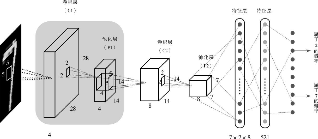
The figure below shows a typical example of a convolutional neural network structure used for handwritten image target detection:

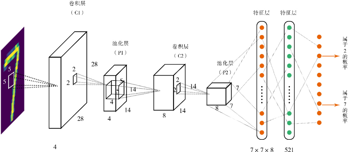
Looking at the structure of the convolutional neural network above, it can generally be divided into four layers:

• Input Layer: The input data is a handwritten image represented by a 2D matrix. Each element in the matrix corresponds to a pixel of the image, and each pixel contains a grayscale value ranging from 0 to 255. The larger the value, the whiter it is; otherwise, the blacker it is.
• Convolutional and Pooling Layers: Corresponding to the two sets of interleaved convolutional and pooling layers in the architecture above, they extract features from the input image step-by-step and reduce their dimensionality, retaining only the important features contained in the image and ultimately outputting them to the feature layer to perform classification tasks.
• Feature Layer: Also known as the fully connected layer, it primarily performs classification tasks based on the outputs of the convolutional and pooling layers. It flattens the features output by the preceding pooling layer into a 1D vector, integrates these recognized global features, and applies activation functions (such as ReLU, Sigmoid, etc.) for non-linear transformation to obtain classification probabilities or predicted values.
• Output Layer: The final output layer contains 10 neurons. For each handwritten image fed into the neural network for recognition, it outputs the recognition probabilities for numbers 0 through 9 across these 10 neurons. The sum of the recognition probabilities for all neurons equals 1. The number corresponding to the highest probability is selected as the output.

The purpose of this article is to explain in detail how the calculation operations unfold in the convolutional and pooling layers after an image enters the CNN through the input layer in the above architecture.

Calculation of the Convolutional Layer

A concept closely related to image convolution is the convolution kernel. A convolution kernel can be thought of as a very small-resolution image. The convolution operation performed on the original image is actually using this small-resolution image (i.e., the convolution kernel) to scan and match pixel by pixel from left to right and top to bottom. The result of the match is a new image, called a feature map. A feature map is a grayscale image where the grayscale value of each pixel represents the degree of match between the original image at that location and the small convolution kernel image, as shown in the figure below:

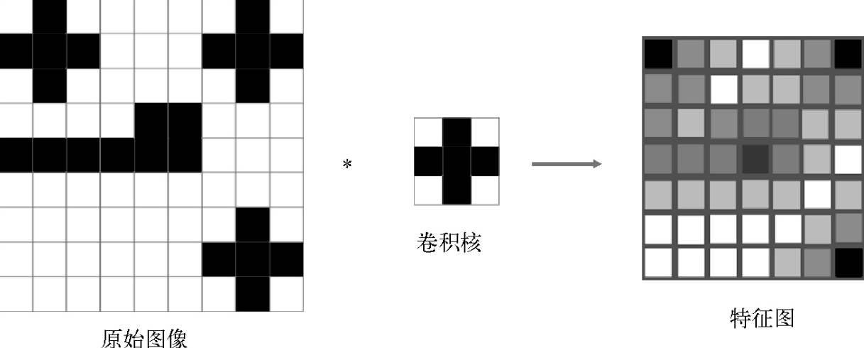
The following figure illustrates the convolution calculation process between the original image and the small convolution kernel image. Here, the convolution kernel is a 3x3 small image, where each pixel is a real value representing the computational weight of the convolutional neural network.

• The weight value corresponding to each pixel in the convolution kernel is the parameter that the subsequent convolutional neural network needs to train.

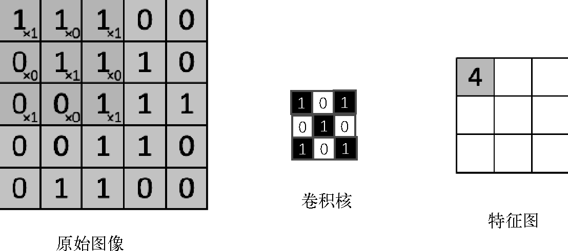
As shown in the figure above, the first step is to perform convolution calculation using the convolution kernel on the top-left corner of the original image. The convolution calculation performed here multiplies each pixel in the 3x3 area of the top-left corner of the original image (which matches the size of the convolution kernel) by the pixel at the corresponding position in the convolution kernel image. Then, the 9 product results in this 3x3 area are added together to obtain the value of the first pixel in the top-left corner of the feature map.

Next, the convolution kernel moves one pixel to the right on the original image and continues the same operation to obtain the value of the second pixel in the first row of the feature map.

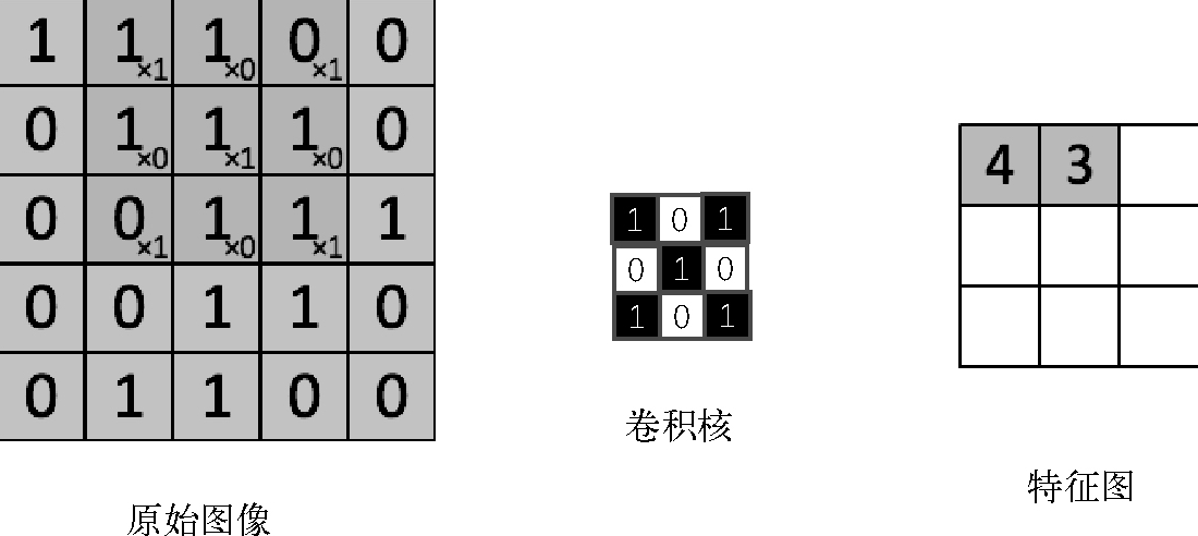
Following the calculation logic above, the convolution kernel is moved to the right sequentially, one pixel at a time, until it reaches the far right of the original image. Then it moves down one pixel to start the convolution for the second row. This process repeats in a loop until the convolution kernel moves to the bottom-right corner of the original image, completing the scan of the entire image and yielding a complete feature map.

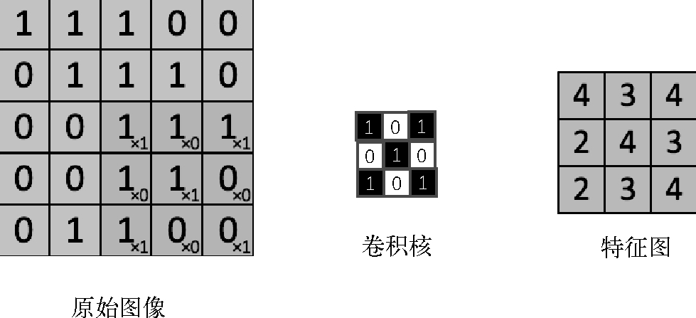
According to the above convolution calculation logic, when the size of the original image is $m \times n$ and the size of the convolution kernel is $w$, the size of the feature map after the convolution calculation is $(m-w+1) \times (n-w+1)$. In other words, the feature map will be slightly smaller than the original image. If you want the feature map size to remain consistent with the original image, you need to pad a border of zeros around the original image before performing the convolution calculation:

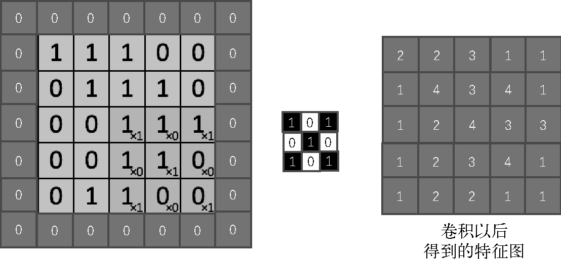
The complete convolution operation performed on the original image using a single convolution kernel yields a feature map corresponding to that convolution kernel. In practice, during the execution of a convolutional neural network, multiple different convolution kernels are often used to independently perform convolution operations on the original image, thereby generating multiple feature maps. For example, the figure below shows convolution operations performed on an original image with a resolution of 125x125 using 100 different convolution kernels, generating 100 feature maps with a resolution of 125x125:

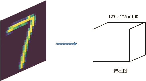
This is also the reason why, in the CNN architecture, the 2D input image turns into a cuboid after passing through the convolution calculation of the first convolutional layer.

Calculation of the Pooling Layer

As shown in the shaded part of the overall CNN architecture below, each convolutional layer is followed by a pooling layer used to simplify the features extracted by the convolutional layer, retaining only the coarse-grained information in the feature map. After convolving the original image with 4 convolution kernels, convolutional layer C1 obtains four 28x28 feature maps. The operation of pooling layer P1 is to perform a pooling operation on each feature map to shrink it, ultimately resulting in four pooled feature maps with a resolution of 14x14. This greatly reduces the data volume while retaining important features.

The pooling operation is very simple. Taking the figure below as an example, the 3x3 pooling operation performed here extracts the pixel with the maximum value from each 3x3 region in the original feature map based on the maximum-value principle, serving as the pooling output for the entire region. In this way, each 3x3 region of the original feature map corresponds to a single pixel in the pooled feature map.

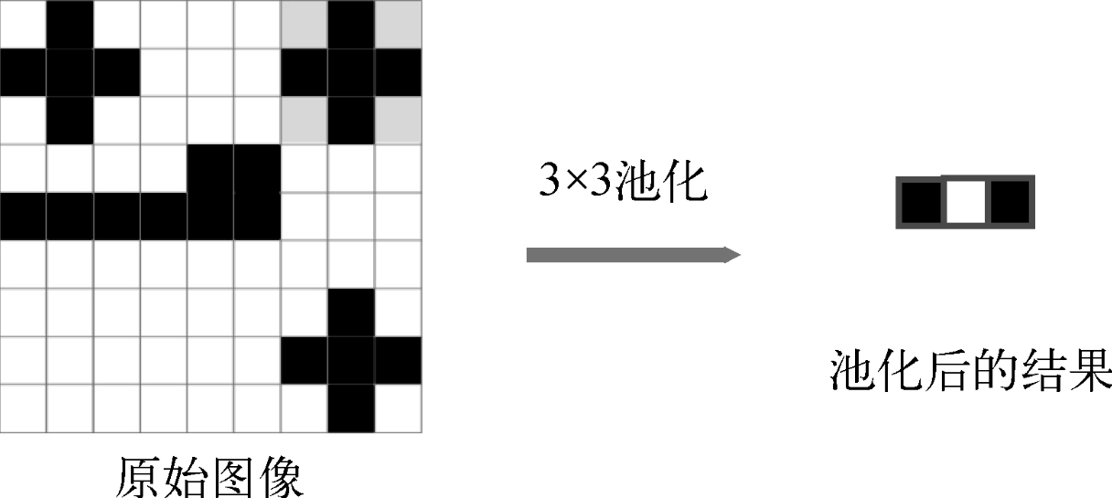
It should be noted that the movement during the pooling operation is non-overlapping, which differs from convolution. Therefore, the output after pooling is much smaller than the original feature map. Consequently, the 9x9 original feature map above, after a 3x3 pooling operation, results in a 3x3 pooled feature map. Similarly, the four original 28x28 resolution feature maps of convolutional layer C1 in the architecture diagram above become four 14x14 resolution pooled feature maps after a 2x2 pooling operation.

3D Convolution Calculation

The output of the pooling layer is a 3D cuboid (multiple pooled feature maps). When this pooled data is fed into the next convolutional layer for calculation, its convolution workflow differs from that when the original image is fed into the first convolutional layer (where the original image is a 2D matrix). When the pooling layer’s output is fed into the next convolutional layer, the required convolution calculation is a 3D convolution calculation.

The figure below shows an example of a 3D convolution kernel. On the left is the pooling layer, and on the right is the next convolutional layer. For the 3D convolution calculation performed on the pooling layer, you must first select a 3D convolution kernel whose depth matches the output of the pooling layer. Then, use this 3D convolution kernel to perform a 3D convolution operation on the multiple pooled feature maps output by the pooling layer. Each operation result (obtained by multiplying corresponding positions across the entire cuboid involved in the 3D convolution operation and then summing them up) corresponds to a single pixel in the convolutional layer. Performing a complete scan of the pooling layer’s output using the 3D convolution kernel corresponds to one feature map of the convolutional layer.

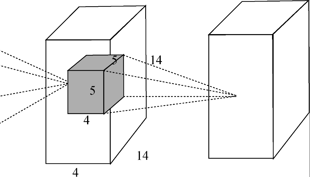
Similarly, there can be multiple 3D convolution kernels. Using one 3D convolution kernel to perform one 3D calculation yields one feature map; thus, the operation results of multiple 3D convolution kernels correspond to multiple feature maps of the convolutional layer. Therefore, the output of the convolutional layer is also a cuboid.

In summary, for a simple convolutional neural network, the calculation workflow of convolution and pooling is: 2D image output -> first-layer convolution calculation (2D convolution) -> first-layer pooling operation -> second-layer convolution calculation (3D convolution) -> second-layer pooling calculation -> second-layer convolution calculation (3D convolution)… This cycle repeats until the image features calculated by convolution are finally organized and passed to the feature layer for the image classification task.

In summary, for a convolutional neural network (CNN), the parameters of its convolutional layers are the parameters within the convolution kernels contained in each convolutional layer. These are the main parameters trained during the CNN training process. Meanwhile, because the pooling layer simply performs 2x2 or 3x3 max-pooling operations, it has no parameters to train.

Reference Materials

• Deep Learning Principles and PyTorch Practice (2nd Edition), Chapter 5: Handwritten Digit Recognizer - Understanding Convolutional Neural Networks
• The Role of Each Layer in Convolutional Neural Networks