Introduction to Audio 3A Processing: AEC, ANS, and AGC

31 Mar, 2025
- Audio & Video

This series of articles provides a comprehensive summary of the concepts, theories, and working principles of 3A audio processing (AGC, AEC, and ANS) in the field of consumer cameras. It lays the foundation for audio effect tuning and troubleshooting in related products.

In the consumer camera domain, similar to the 3A processing in video and imaging—namely AE (Auto Exposure), AWB (Auto White Balance), and AF (Auto Focus)—there is a corresponding 3A processing framework for audio data, known as Audio 3A: AGC (Auto Gain Control), AEC (Acoustic Echo Cancellation), and ANS (Auto Noise Suppression). The purpose of this article is to summarize the theoretical technologies and operational workflows of these audio 3A processes.

The following diagram illustrates a typical audio 3A processing workflow for two-way voice communication with a remote end via a server:

The data captured by the microphone is first processed alongside the received remote voice data to identify echoes, and the AEC (Acoustic Echo Cancellation) algorithm is applied to eliminate them.
Next, the echo-cancelled voice signal passes through the ANS (Auto Noise Suppression) module to filter out audio noise and improve the quality of the captured audio.
AGC is then used to dynamically and adaptively adjust the audio gain according to the amplitude of the captured voice, bringing the signal strength transmitted to the remote end to an appropriate level.
The raw audio data is encoded and transmitted over the network and server to the remote end of the voice communication.
Upon receiving the voice information, the remote end organizes the audio data using various buffering and packet-loss retransmission mechanisms.
The remote end decodes the received compressed audio data to restore the raw audio format.
Finally, combined with local mixing and other settings, the raw audio data is played out through the speaker.

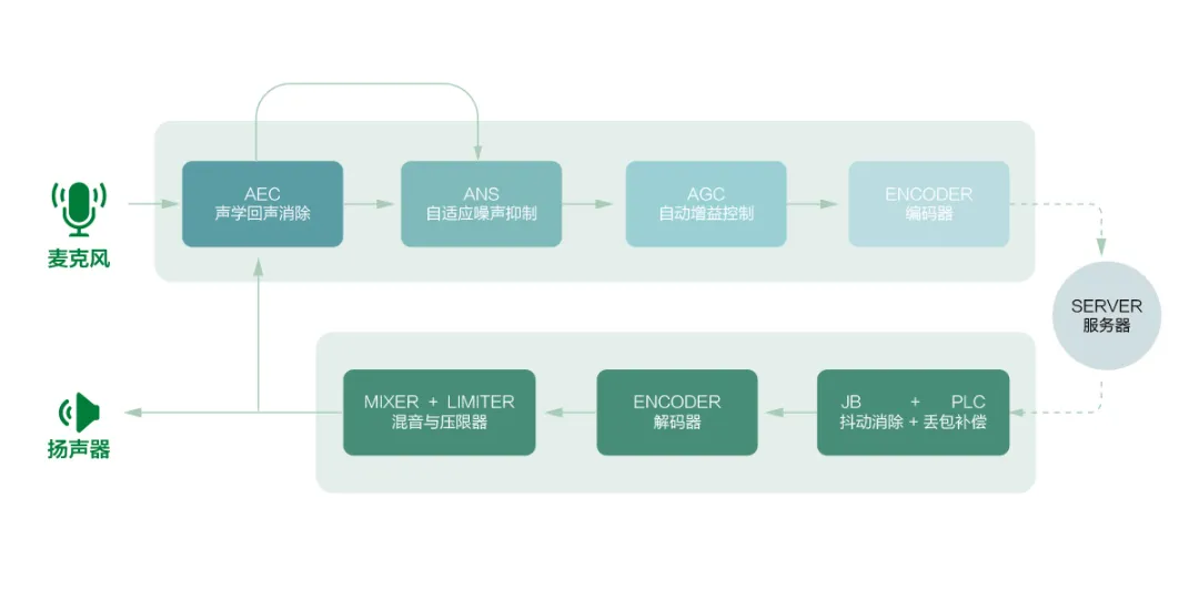
Overall, in a full-duplex two-way audio intercom application, the general processing order for audio 3A is: AEC (Acoustic Echo Cancellation) first, followed by ANS (Audio Noise Suppression), and finally AGC (Auto Gain Control).

Acoustic Echo Cancellation (AEC)

The problem that AEC aims to solve is that during a two-way voice call (such as a conference call), the sound emitted by the speaker at one end (originating from the other end) is captured by the microphone at the same end and transmitted back to the opposite end. This causes the voices of both parties to bounce back and forth, creating a noticeable echo effect.

The diagram below illustrates how echoes occur in two-way full-duplex voice calls and conference calls:

As seen from the diagram illustrating the generation principle of two-way call echoes, echo problems only occur during two-way full-duplex voice calls (where both the microphone and speaker at both ends remain active). In half-duplex systems (similar to walkie-talkies), echoes and echo cancellation are non-existent. This is because, in half-duplex voice communication, only one party’s microphone is open at any given time. Furthermore, a user always listens to the other party first before pressing the talk button to send their own voice. Consequently, whenever a party’s microphone is open, their own speaker is silent, naturally eliminating the presence of echoes and the need for echo cancellation. Of course, this communication mode is relatively inefficient since only one person can speak at a time.

In practical echo cancellation application scenarios, echoes are often categorized into two types based on their propagation paths:

Direct Echo: Also known as linear echo. This occurs when the voice signal transmitted from the remote end is played out through the local speaker and directly captured by the local microphone without undergoing any reflection or refraction. This type of direct echo is unaffected by the environment and depends solely on the distance and position between the local microphone and speaker, making the time delay of the echo relatively easy to estimate.
Indirect Echo: Also known as non-linear echo. This occurs when the remote voice signal played through the local speaker reflects and refracts off various obstacles, walls, and floors in the local environment before being captured by the local microphone. Therefore, the magnitude of indirect echo is related to the room environment, layout, and even the sound absorption coefficients of various obstacles. When the communication device itself is moving, the positions of the speaker and microphone relative to the environmental obstacles are constantly changing, resulting in a dynamically varying echo delay. Consequently, this type of echo is relatively difficult to handle.

Processing Logic of Echo Cancellation

From the perspective of how echoes are generated, consider two communicating parties, A and B. A’s voice signal is captured by A’s microphone and transmitted to B. After being played out by B’s speaker, it is re-captured by B’s microphone and mixed with B’s own voice signal before being sent back to A. As a result, A hears their own voice coming out of their speaker. Therefore, throughout this process, party A is innocent; the echo problem arises because B’s microphone captures both its own voice signal and A’s voice signal played by the speaker, mixing them together and sending them to A without any processing, which causes the echo at A’s end.

Therefore, solving the echo problem must start at party B’s end. After capturing the audio data, B’s end must identify and separate its own voice signal from A’s voice signal being played by the speaker, eliminate A’s voice signal from the mixed audio data, retain only its own voice signal, and then transmit it to A. This is the exact logic behind introducing the AEC echo cancellation module at party B’s end.

Of course, because party A and party B are engaged in full-duplex two-way voice communication where both sides are symmetrical, in practice, AEC echo cancellation functions and modules need to be implemented simultaneously at both ends. Each module identifies and eliminates the remote voice signal (played by its own speaker) from the mixed signal captured by its local microphone.

Working Principle of Echo Cancellation

As mentioned above, echo cancellation involves identifying the remote voice signal (played by the local speaker) within the mixed signal received at the microphone and eliminating it, ensuring that only the local raw voice signal is transmitted to the other end. To meet this design requirement, an echo cancellation module generally consists of the following four sub-modules.

1. Delay Estimation Module

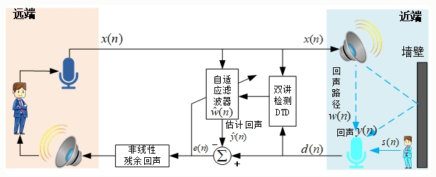
To eliminate the remote voice signal played by the speaker, the system must first identify this signal within the mixed signal captured by the local microphone and determine the time difference between the remote voice signal played by the speaker and the voice signal captured by the local microphone. With this time difference, subsequent processing modules can accurately locate the remote voice signal that needs to be attenuated within the microphone-captured data.

How is the time difference between the two voice signals (the received remote voice signal data and the local microphone-captured voice signal data) determined? The answer is to slice both voice signals, perform a Fourier transform on each sliced audio data frame to obtain their spectral data, and then compare their similarities in the frequency domain using cross-power spectral calculations until the slice where the spectral behavior of both audio data sets matches best is found. This identifies the time difference.

2. Linear Echo Cancellation Module Based on Adaptive Filters

This module is the core of the entire echo cancellation system.

In the practical implementation of the echo cancellation algorithm, the locally received remote voice data is used as input. Through dynamic iteration and updating of the filter weight parameters of the adaptive filter, its output signal is made as close as possible to the actual echo signal data. Finally, the predicted echo data output by the adaptive filter is subtracted from the mixed signal captured by the microphone, achieving the goal of preserving pure local voice data.

3. Non-linear Residual Echo Suppression Module

The linear echo cancellation module implemented using adaptive filters described above can only eliminate the linear echo components of the acoustic path and cannot completely eliminate non-linear distortion. Therefore, after filtering out the linear echoes using the adaptive filter, a non-linear module must be employed to further suppress residual non-linear echoes through techniques such as frequency-domain energy analysis and dynamic gain control.

4. Double-Talk Detection Module

This module dynamically monitors the remote voice data and the voice data captured by the local microphone to determine whether only one party is speaking or both parties are speaking simultaneously.

If both parties are talking at the same time, the audio data captured by the local microphone will contain the voice signals of both parties. In this case, the local voice signal might be misjudged as residual echo, leading to incorrect updates of the filter parameters. Therefore, when the algorithm identifies that both parties are in a double-talk state via the double-talk detection module, it freezes the updating of the filter weights to prevent the algorithm from diverging due to noise interference.

Conversely, when the double-talk detection module detects that only one party is speaking, it can resume updating the adaptive filter weights and increase the echo suppression intensity of the filter to completely eliminate residual echoes, thereby achieving a better intercom effect.

Referencing the diagram below helps in better understanding the complete implementation of the echo cancellation algorithm and the roles played by its sub-modules in the overall echo cancellation workflow.

Auto Noise Suppression (ANS)

The raw sound signals captured by microphones in commonly used products like smartphones and consumer cameras often contain a significant amount of background noise. This not only degrades the user experience during recording and playback but also reduces the compression efficiency of audio encoding. Therefore, suppressing audio background noise is necessary, which is where the ANS (Auto Noise Suppression) function comes into play.

In addition to the aforementioned ANS technology, audio 3A also includes ANC (Active Noise Cancellation) for controlling environmental noise. The main difference between ANS and ANC lies in their approach: the former adopts a passive noise reduction method, analyzing frequency components in environmental noise to perform targeted filtering, preserving the clear voice part as much as possible and improving sound quality. The latter, commonly found in popular active noise-canceling headphones currently on the market, analyzes the frequency and phase of environmental noise sound waves to generate sound signals with opposite phases to achieve noise cancellation. Therefore, the primary difference is that ANS uses passive filtering for noise reduction, whereas ANC actively generates waveforms with opposite phases to the noise to cancel each other out. Generally speaking, in the consumer camera domain, only ANS is used for processing sound data captured by camera microphones; hence, this article focuses solely on the passive noise reduction mechanism of ANS.

Sources of Audio Background Noise

Generally speaking, in analog systems, noise can originate from various stages of the system, making analog systems more susceptible to interference and noise generation. For digital devices, anti-interference and noise performance are much better, with the weak links for noise ingress typically being the A/D and D/A conversion sections. In the consumer electronics sector, considering factors such as cost, analog audio components and processing circuits remain mainstream in applications. Consequently, sound quality degradation caused by background noise from various disturbances in these products often presents a major challenge in product development.

In general, the audio noise in consumer camera products primarily originates from the following aspects:

Inherent noise during the operation of electronic components. For example, electronic components (capacitors, resistors, etc.) operating at high frequencies inherently generate subtle white noise. These noises are easily picked up by nearby high-sensitivity microphones, amplified, and made clearly audible.
Electromagnetic interference. During the high-frequency switching operation of circuits—especially when wireless communication circuit functions operate within the internal space of the device—high-frequency electromagnetic wave radiation interference leaks into the analog audio signal via audio transmission lines, generating electromagnetic interference noise.
Power supply interference and ground loop noise. Spikes, pulses, and surges in the power supply circuit leak into the audio lines via power paths, and ground potential differences between different circuit sections cause current loops. These power and ground noises have a significant impact on small analog audio signals.

As seen from the summary of audio noise sources above, most of these audio noises originate from the design and implementation of hardware devices. Some noise sources can be optimized—for example, by optimizing power grounding design and adjusting layout to improve electromagnetic interference conditions in audio routing modules. However, it is undeniable that structural and electronic design limitations in consumer electronics products can cause some interference factors to not be completely resolved at the hardware level. In such cases, methods must be devised to utilize audio enhancement features within the Audio Codec or even software-level audio noise filtering algorithms to improve the quality of audio capture.

Typical Classification and Processing of Noise

In general, audio background noise can be divided into two categories: stationary noise and transient noise.

The primary characteristic of stationary noise is that its statistical properties (such as mean, variance, and spectral distribution) do not change over time.

In the time domain, stationary noise exhibits small amplitude fluctuations and displays a regular distribution (such as a Gaussian distribution).
In the frequency domain, its spectrum is continuous and stable; for example, white noise covers the entire frequency band.
Typical stationary noise scenarios include: Gaussian white noise, thermal noise of electronic devices, quantization noise, and continuous background environmental noise (such as air conditioner hum or fan noise).

Transient noise, on the other hand, is highly bursty and short-lived (ranging from milliseconds to seconds), and its statistical properties generally change drastically over time.

In the time domain, transient noise typically features high amplitude and short-duration impulse characteristics.
In the frequency domain, its energy is generally concentrated in high frequencies or specific frequency bands.
Typical transient noises include impulse noise (keyboard typing, door knocking, switching sounds), mechanical shock sounds, and irregular electromagnetic interference (such as electrostatic discharge).

Generally speaking, stationary noise is relatively easy to handle because its statistical properties and spectral distribution are relatively stable and easy to recognize, allowing for targeted suppression based on its spectral characteristics and specific signal features. However, transient noise exhibits strong burstiness in the time domain, and its spectrum almost always overlaps with that of normal speech, making it very difficult to suppress. Consequently, there is currently a lack of good technical solutions for effectively suppressing transient noise.

Typical Audio Noise Reduction Algorithms: Spectral Subtraction and Adaptive LMS Filtering

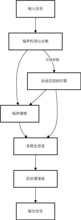
The figure below shows the processing flowchart of a typical audio noise reduction algorithm. Whether using traditional signal processing algorithms or AI-enhanced processing approaches, the ultimate goal is to detect the type of audio noise, model the noise, and then perform targeted processing based on the noise model.

Below, two commonly used traditional digital signal processing algorithms for audio noise reduction—Spectral Subtraction and Adaptive LMS Filtering—are explained and illustrated.

Spectral Subtraction

Spectral subtraction is a frequency-domain-based noise suppression technique. It estimates and models the noise spectrum and subtracts the noise components from the noise-containing mixed signal in the frequency domain. Since it is a frequency-domain-based processing method, the overall processing workflow inevitably involves using the FFT (Fast Fourier Transform) to convert the time-domain audio sample data sequence into a frequency-domain spectral sequence, processing it in the frequency domain, and then converting the processed signal back to the time domain using the IFFT (Inverse Fast Fourier Transform). Such a processing workflow naturally involves a significant amount of computation.

The overall working principle of spectral subtraction is to estimate and establish a noise power spectrum template during voice silence periods (i.e., time intervals containing only noise), and then subtract the power spectrum of the noise template from the power spectrum of the noise-containing mixed signal, thereby achieving the goal of retaining only the speech components.

The workflow for audio noise cancellation based on spectral subtraction is roughly as follows:

First, slice the time-domain audio sampling data sequence. The slice duration is fixed and matches the number of points for the FFT calculation. For example, with a 16 kHz audio sampling rate and a 512-point FFT calculation, audio data is sliced into units of 32 ms, where each audio slice unit constitutes an audio frame.
Perform an FFT calculation on this audio frame to obtain its spectral data.
Use an independent VAD (Voice Activity Detection) module to detect whether the current period is a speech silence period. When in a silence period, dynamically update the noise power spectrum template based on the spectral sequence currently calculated via FFT, making it consistent with the current noise spectrum state.
Perform spectral subtraction in the frequency domain on the spectral data sequence of the current audio frame: subtract the power spectrum of the current noise power spectrum module at the corresponding frequencies from the spectral data of the current audio frame, yielding frequency-domain data that retains only the speech components.
Finally, convert the processed data back from the frequency domain to the time domain using IFFT, re-combining it into an audio data sequence to restore the continuous time-domain audio sampled signal.

Adaptive LMS Filtering Algorithm

Unlike spectral subtraction, which operates in the frequency domain, the LMS (Least Mean Squares) filtering algorithm is an adaptive filter algorithm operating in the time domain. It dynamically compares the real-time audio sampled data sequence with the filter’s output and iteratively adjusts the filter coefficients based on the calculated error to minimize the mean square error between the desired signal and the filter’s output.

The adaptive LMS filter primarily has two parameters:

Filter Order ( $L$ ): The length of the noise used for modeling, which matches the time correlation of the noise. A larger $L$ means that filtering each audio sample will reference more historical sampling data, resulting in a higher computational load. Typical values range between 64 and 256.
Step Size ( $\mu$ ): Primarily used to control the convergence speed and stability of noise change tracking, with typical values ranging between 0.001 and 0.01.

Execution workflow of the adaptive LMS filtering algorithm:

First, place the current input audio sampling data to be filtered, along with the $L-1$ historical audio sampling data preceding this sample, into a buffer named History.
Based on the historical buffer data and the current parameters $W$ of the LMS filter, calculate the output value $Y$ of the LMS filter: accumulate the products of the historical sampling data History[i] and the filter parameters W[i].
Calculate the difference $E$ between the current audio sampling data input and the calculated LMS filter output $Y$ . This difference $E$ represents the value filtered by the LMS adaptive process.
Update the operating parameters $W[i]$ of the filter system based on the difference $E$ , the sampling data History[i] in the history buffer, and the step size $\mu$ of the LMS filter.
Return the calculated difference $E$ .

Below is a reference code snippet for processing with the adaptive LMS filtering algorithm, which can be used to understand the execution workflow above:

#define L 128  // Filter order is 128
#define FRAME_SIZE 256
#define MU 0.002f   // Step size mu is 0.002f

float w[L] = {0};          // Filter coefficients
float x_history[L] = {0};  // History buffer for audio sampling data

void process_frame(float *input, float *output) {
    for (int n = 0; n < FRAME_SIZE; n++) {
        // 1. Update input history (FIFO)
        // Place the latest audio sampling data at the beginning of the x_history buffer each time
        memmove(x_history + 1, x_history, (L-1)*sizeof(float));
        x_history[0] = input[n];

        // 2. Calculate filter output y
        float y = 0.0f;
        for (int i = 0; i < L; i++) {
            y += w[i] * x_history[i];
        }

        // 3. Calculate error e, which is effectively the filtering operation
        float e = input[n] - y;

        // 4. Update filter coefficients
        for (int i = 0; i < L; i++) {
            w[i] += MU * e * x_history[i];
        }

        // 5. Output noise-reduced result
        output[n] = e;
    }
}

In practical applications, the LMS adaptive filtering algorithm is often combined with dual microphones to achieve better noise reduction results. The primary microphone is placed close to the human mouth to capture the speaker’s voice, while the secondary microphone is placed far from the mouth and close to the noise source (such as the outside of a headset) to capture environmental noise. During operation, the environmental noise data captured by the secondary microphone is used to train and update the parameters of the LMS filter, which then filters the audio sampling data from the primary microphone. This approach yields exceptional suppression effects on periodic noise (such as engine or fan noise).

Of course, if dual microphones are used, the execution workflow and corresponding code of the LMS filtering algorithm above need to incorporate a sampling sequence of a reference audio signal (from the secondary microphone). The calculations for History, the output of the LMS filter, and its parameter updates are based on the sampling data of the secondary microphone, while the filtering of the primary microphone’s sampling data is performed by subtracting the LMS filter output from the primary microphone’s sampling data.

Comparing the implementations of spectral subtraction and adaptive LMS filtering algorithms, spectral subtraction involves two mutual conversions between the frequency domain and the time domain, resulting in a relatively high computational load, though it processes one block of operations per audio frame. On the other hand, the adaptive LMS filtering algorithm performs calculations directly in the time domain, but requires two floating-point operations equal to the filter order for every single sample—one for calculating the filter output and one for updating the filter’s operating parameters. Therefore, if the filter order is high, the computational load can also be significant. Overall, however, the latter has lower demands on computing resources and is more suitable for resource-constrained embedded systems.

Audio Auto Gain Control (AGC)

In audio calls and video conferencing, the primary functions of the Audio Auto Gain Control (AGC) module are:

To stabilize the output level of the audio signal. Regardless of the strength of the signal captured by the microphone (e.g., varying distances of users from the microphone), AGC strives to ensure that the output volume of the audio capture module remains relatively consistent, preventing clipping caused by excessively high volume or inaudibility caused by excessively low volume.
To dynamically adapt to changing environments in volume capture. This includes coping with environmental noise variations, device differences (such as different microphone sensitivities), and differences in user speaking habits, automatically and dynamically adjusting the strength of the voice signal to keep its output at an appropriate level.

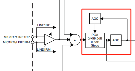
In the processing chain of typical consumer electronic Audio Codecs, the AGC module generally operates in the digital domain after ADC conversion, implementing the function of dynamically adjusting the gain of voice signal data via DSP algorithms. This processing approach offers better flexibility and allows for collaborative optimization with other DSP algorithms such as noise reduction and AEC. Of course, some low-end Audio Codecs (such as the TLV320AIC3101) lack rich digital audio processing functions internally; in such cases, the AGC module can also directly adjust the PGA gain in the analog domain to achieve auto gain control. The diagram below shows the AGC processing chain of the TLV310AIC3101.

Additionally, AGC dynamic gain adjustment is only used in the input processing chain of the audio signal—namely, the processing of voice signals captured by the microphone—to achieve a basically consistent voice signal strength. In the output processing chain of the audio signal, which is the processing chain for playing voice signals through speakers, AGC is generally unnecessary. The volume of the output voice signal is typically managed manually by the user or controlled via system volume management, requiring no automatic gain.

AGC Audio Processing Chain and VAD Module

Generally speaking, the sound signal captured from the microphone inevitably contains a certain amount of noise and echoes from two-way intercom states, in addition to the local voice signal we actually want to preserve. Since AGC maintains volume stability by adjusting the gain of audio sampled data, the object of its stabilization must inevitably be the local voice signal with noise and echoes removed as much as possible. This is why AGC should be placed after AEC and ANS in the audio 3A processing chain, as the objects for which we perform auto gain control should not include echoes and noise.

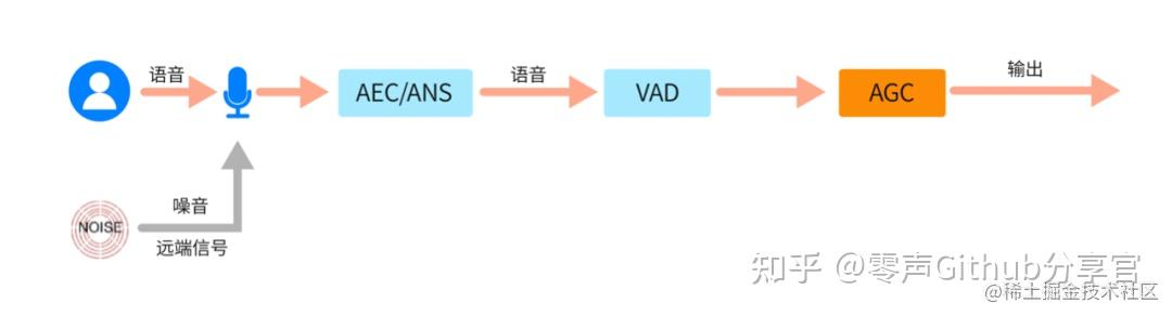
After the aforementioned noise and echoes are processed by the ANS and AEC stages respectively, the AGC auto gain control processing workflow also incorporates a VAD (Voice Activity Detection) module to determine when to initiate gain adjustment for the audio sampled data. The primary objective of the VAD module is to distinguish continuous voice signals captured by the microphone into speech segments and non-speech segments (such as silence or background noise). AGC is activated to dynamically control the gain of audio data only during speech segments, while gain adjustment is suppressed or maintained at a fixed gain during non-speech segments. This prevents amplifying noise and avoids negative impacts of AGC’s dynamic gain adjustment on non-speech signals.

The VAD module’s decision on speech and non-speech segments operates on a per-audio-frame basis. It calculates the root-mean-square (RMS) energy of the audio sampled data within the frame and compares it with the dynamic local noise energy maintained by the VAD module. If the energy of the current frame is higher than the dynamic noise floor plus a fixed offset (e.g., +3 dB), it can be determined as a speech segment candidate. Combined with a state machine control mechanism (such as determining a speech segment when multiple consecutive frames exceed the threshold, and a non-speech segment when multiple consecutive frames fall below it), the final verdict for speech and non-speech segments is rendered.

AGC Processing Workflow

1. Preprocessing of Audio Sampled Data

As mentioned above, AGC operates in the digital domain of the Audio Codec, executing auto gain processing on the digital sampling sequence captured by the microphone after ADC conversion and other audio processing modules. In this stage, continuous audio sampled data is first sliced into audio frames containing a fixed number of samples, and subsequent AGC processing is performed on a per-audio-frame basis.

Frame-based processing in AGC typically employs a 50% overlap method, meaning the first 50% of samples in the current audio frame are identical to the last 50% of samples in the previous audio frame. This smooths out boundary effects between audio frames and prevents sudden jumps caused by different gains in two consecutive audio frames.

2. VAD Detection

As noted above, the VAD module determines whether the current audio frame is in a speech segment or a non-speech segment by comparing the frame energy of the current audio with the noise floor energy.

AGC gain adjustment is generally triggered only during speech segments within the AGC workflow.

3. Auto Gain Calculation Phase

The auto gain calculation phase relies on several preset values of the AGC module:

Target Level: The target volume level that the AGC module expects its output to reach.
Time Constant: The time parameter for gain adjustment, used to control the smoothness of gain regulation and prevent abrupt volume fluctuations.

When calculating the gain, the energy of the current audio frame is compared with the target level. If the energy of the current frame is higher than the target level, the gain is appropriately reduced to prevent overloading after the audio sampled data is combined with the gain. Conversely, if the energy of the current frame is lower than the target level, the gain is increased to raise the volume amplitude.

For application scenarios with a relatively small signal dynamic range (where differences in signal amplitudes are minor), a linear gain adjustment mode can simply be selected: a gain magnitude is determined based on the difference between the current audio frame’s energy and the target level, and the same gain adjustment is applied to all audio samples.

For complex signal environments (such as burst noise and multi-band interference), a non-linear gain adjustment strategy must be adopted:

Dynamic Range Control (DRC). DRC is a technique that adjusts the signal dynamic range through non-linear gain adjustment, widely used not only in voice signal processing but also in communication systems and smart devices. DRC operation roughly relies on three parameters: threshold_low, threshold_high, and ratio. Its working logic is generally: when the amplitude and energy of the audio samples are below the threshold_low threshold, DRC sets a relatively low gain to suppress noise; when the amplitude and energy of the audio samples are between threshold_low and threshold_high, DRC sets the gain for the audio samples according to the target gain calculated previously; and when the amplitude and energy of the audio samples are greater than threshold_high, the gain for the audio samples is appropriately compressed according to the ratio setting to prevent clipping.
Multi-band Gain Control. Band splitting is first performed via FFT calculations to divide the signal into low-frequency, mid-frequency, and high-frequency sub-bands. Then, gain is calculated and adjusted independently for each sub-band. This avoids spectral imbalance caused by overall adjustment. The entire processing approach is somewhat similar to the workflow of an equalizer (EQ), setting different gains for different frequency bands to suppress or enhance them.

In addition, the time constants for automatic gain calculation and adjustment mainly consist of two types of time parameters used to achieve smooth and natural changes in gain and adjusted voice amplitude:

Attack Time: Rapidly reduces gain (typical value 20–100 ms) when the amplitude of the audio signal suddenly surges, preventing transient overload issues.
Release Time: Slowly restores gain (typical value 100–2000 ms) when the signal amplitude weakens.

4. Gain Application Phase and Post-Processing

The final stage of AGC processing applies the gain calculated during the calculation phase to all sample data within the current audio frame. Depending on whether a linear or non-linear gain calculation strategy was adopted in the previous stage, consistent or varying gains are applied to the audio samples accordingly.

Additionally, the audio sample sequence data processed by AGC must also have its amplitude limited (e.g., to -1 dBFS) to prevent DAC or speaker overload, and it requires feedback coordination with audio processing modules from previous stages, such as AEC and ANS, to achieve stable control over the audio data.