Detailed Explanation of the G.711 Audio Compression Standard

G.711 is an audio compression standard defined by the ITU-T, widely used in telecommunication networks and VoIP fields. In practical implementation, G.711 audio encoding and decoding can be divided into two formats: μ-law (mainly used in North America and Japan) and A-law (mainly used in Europe and the rest of the world), both of which are explained in detail in this article.

The sampling rate defined by G.711 in telephony applications is 8kHz (One point that needs to be clarified is that the G.711 audio encoding algorithm itself does not restrict the sampling rate. The 8kHz sampling rate here is a compatibility requirement of telephone communication networks. Therefore, if compatibility between equipment from different manufacturers in a call system must be considered, the standard-defined 8kHz should be used. However, if G.711 is only used to encode and decode audio data at both ends of the communication without needing to consider compatibility with other manufacturers’ equipment, a higher sampling rate can absolutely be adopted.). Each audio sample produces a 16-bit raw sample. In this case, the bitrate of the raw data is 8000Hz x 16bit = 128Kbps. The G.711 audio encoding algorithm encodes this raw audio sample data, compressing each 16-bit audio sample into 8 bits, yielding a compression ratio of 2:1. Consequently, it produces 64Kbps of encoded data for an 8kHz sampling rate.

As mentioned above, there are two primary encoding methods in the concrete implementation of the G.711 audio codec: μ-law (used in North America and Japan) and A-law (used in Europe and other regions). Both μ-law and A-law are non-linear quantization methods. During audio data encoding, logarithmic compression is used to optimize the dynamic range, which provides higher precision at lower volumes and lower precision at higher volumes.

Theory and Implementation of G.711 A-law

The theoretical formulas for G.711 A-law encoding and decoding of audio sample data are shown below. Here, A generally takes a constant value of 87.6, and sgn(x) is the sign function, returning 1 when x is positive and -1 when negative. x is the normalized value of the audio sample data between (-1, 1). Specifically, the highest bit of each 16-bit audio sample is the sign bit; before calculating according to the formula below, the 15-bit data excluding the sign bit is divided by 32768, and then combined with the sign bit to obtain the normalized data in (-1, 1).

Encoding formula:

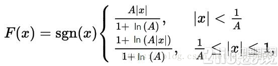
Decoding formula:

The figure below shows the mapping between the normalized audio sample data and the A-law encoded data drawn according to the above formulas. As we can see, when the audio sample value x is relatively small, the variation of its mapped F(x) in the figure is very steep—a slight change in x leads to a drastic change in F(x). Therefore, when the sample value is small, A-law encoding has higher precision. Conversely, when the sample value is relatively large, the rate of change of F(x) is much smaller, meaning the sampling precision is relatively coarser.

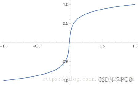
The code implementation of the G.711 A-law audio encoding process described above is as follows:

#include <stdint.h>
#include <math.h>

// 归一化函数
float normalize_16bit_to_float(int16_t sample) {
    return (float)sample / 32768.0f;
}

// A-law量化函数
uint8_t a_law_encode(float sample) {
    const float A = 87.6f;
    float sign = (sample >= 0) ? 1.0f : -1.0f;
    sample = fabs(sample);
    float compressed;
    if (sample < 1.0f / A) {
        compressed = sign * (A * sample) / (1.0f + log(A));
    } else {
        compressed = sign * (1.0f + log(A * sample)) / (1.0f + log(A));
    }
    // 将压缩后的值映射到8位
    return (uint8_t)((compressed + 1.0f) * 127.5f);
}

In the concrete implementation, normalize_16bit_to_float is first called to perform the normalization calculation of the audio sample data, normalizing the 16-bit sample data to range between (-1, 1). Then, a_law_encode is called for encoding, and the encoding result is an unsigned single-byte data.

However, performing A-law encoding and decoding calculations according to the theoretical formulas involves logarithmic operations like log, which posed a major challenge for early telephone systems in the telecommunication field due to limited hardware resources. Therefore, in the actual implementation of A-law, to save valuable computing resources, the 13-segment piecewise linear approximation (13-segment A-law curve) is generally adopted to approximate the theoretical A-law curve and reduce computational complexity. The 13-segment method segments the dynamic range of the input signal into multiple intervals, approximating each interval with a straight line. This approach preserves the non-linear characteristics of A-law while greatly reducing computational complexity.

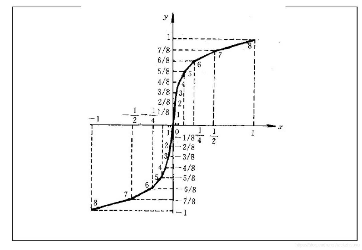
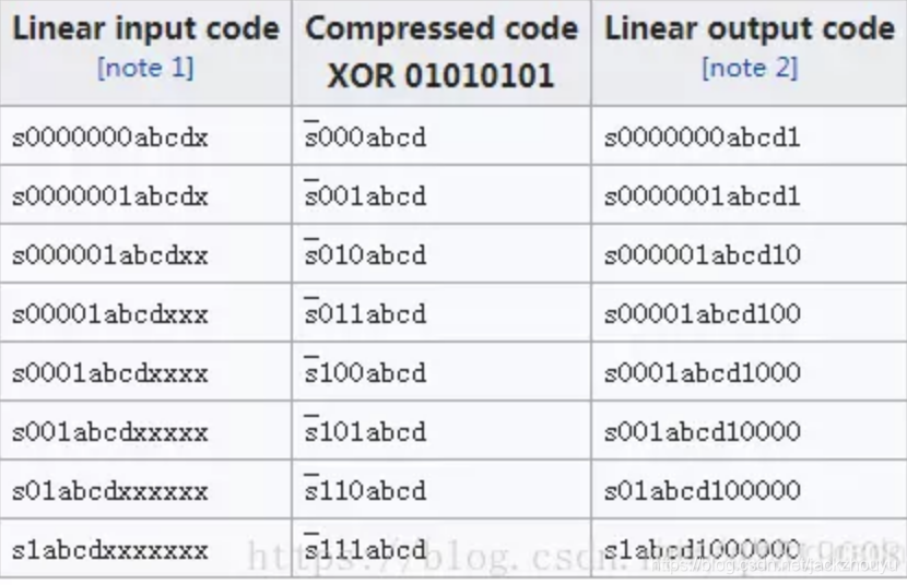
When performing A-law operations using the 13-segment method, the 16-bit audio sample data is first right-shifted by 3 bits to become 13-bit data. Then, this 13-bit data undergoes the following calculations to obtain the sign bit (1 bit), exponent part (3 bits), and mantissa part (4 bits) respectively, which are finally combined into an 8-bit data:

• First, take the highest bit of the 13-bit data as the sign bit. Invert it to get s;
• By examining the remaining 12-bit data, determine the value of the exponent part based on the position of the highest occurrence of a “1” bit, ranging from 0b000 to 0b111 (i.e., the exponent bits eee);
• Extract four bits to the right from the highest “1” bit position of the 12-bit data to get the mantissa bits abcd;
• Finally, combine the sign bit, exponent bits, and mantissa bits into seeewxyz, completing the encoding.

The above workflow is illustrated in the figure below:

Below is a code snippet for compressing 16-bit audio samples using G.711 A-law.

unsigned char linear2alaw(int16_t pcm_sample) {
    int sign, exponent, mantissa;

    // 取符号位
    sign = (pcm_sample < 0) ? 1 : 0;
    pcm_sample = (pcm_sample < 0) ? -pcm_sample : pcm_sample;

    // 归一化：将 16 位 PCM 数据右移 3 位，使其范围适应 13 折线法
    pcm_sample >>= 3;

    // 计算指数部分（段号）
    exponent = 0;
    while ((pcm_sample >> (exponent + 4)) > 0) {
        exponent++;
    }

    // 计算尾数部分（段内偏移）
    mantissa = (pcm_sample >> exponent) & 0x0F;

    // 组合 A-law 编码值
    unsigned char alaw_sample = (sign << 7) | (exponent << 4) | mantissa;

    return alaw_sample;
}

Theory and Implementation of G.711 μ-law

The G.711 μ-law compression algorithm is mainly used in North American and Japanese markets. The theoretical encoding formula is as follows:

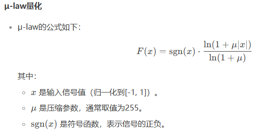
• Before performing the above calculation, the 16-bit sample data must still be normalized to the range (-1, 1), just like in A-law.
• The input for the above formula is the 16-bit audio sample data normalized to (-1, 1), and the output is the compressed 8-bit encoded data generated from the audio sample.

The decoding formula is shown in the figure below:

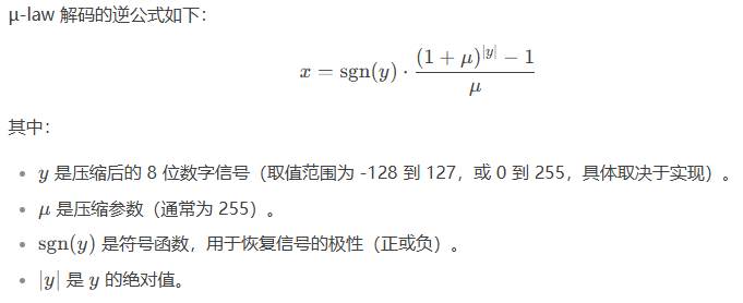
• The input of the above calculation formula is the 8-bit compressed data generated by G.711 encoding, and the output is the decoded data in the range of (-1, 1). To actually play it, it needs to be re-mapped into 16-bit audio sample data and played through an audio codec.

The concrete implementation of G.711 μ-law is similar to that of A-law, also utilizing a piecewise linear approximation method to approximate the μ-law curve to reduce computational overhead. The difference is that A-law uses a 13-segment approximation, where the input to the segment calculation is 13-bit data obtained by right-shifting the audio sample by 3 bits. In contrast, μ-law uses a 15-segment approximation, and the input for the segment calculation is 14-bit data obtained by first right-shifting the audio sample data by 2 bits.

The workflow of the 15-segment approximation can be implemented using a lookup table based on the table below:

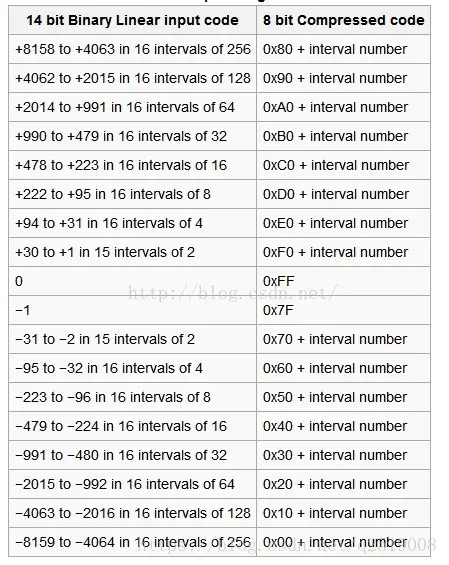
Taking an audio sample value of 1234 (after being right-shifted by 2 bits) as an example, the specific lookup process for the 15-segment approximation is explained as follows:

• First, find the range interval by querying the table above. Looking up the table shows that 1234 lies in the following interval: +2014 to +991 in 16 intervals of 64
• Based on the above interval range, we get its base value as 0xA0 and the interval size (interval) as 64.
• The initial value of the above interval range is 2014. The difference between the current value 1234 and the initial value of the interval range is 2014 - 1234 = 780.
• Calculate the offset based on the above difference: 780 / interval = 780 / 64, yielding 12 after truncation.
• The final output obtained is 0xA0 + 12 = 0xAC.

You can refer to the following code implementation:

#include <stdint.h>
#include <stdio.h>

#define BIAS 0x84  // μ-law 偏移量
#define CLIP 8159  // 最大量化级数量

static int seg_uend[8] = {0x3F, 0x7F, 0xFF, 0x1FF, 0x3FF, 0x7FF, 0xFFF, 0x1FFF};

// 查找段号
static int search(int val, int *table, int size) {
    int i;
    for (i = 0; i < size; i++) {
        if (val <= table[i]) {
            return i;
        }
    }
    return size;
}

// μ-law 编码函数
unsigned char linear2ulaw(int16_t pcm_sample) {
    int mask, seg, uval;

    // 右移 2 位，保留高 14 位数据
    pcm_sample = pcm_sample >> 2;

    // 符号位处理
    if (pcm_sample < 0) {
        pcm_sample = -pcm_sample;  // 负数取绝对值
        mask = 0x7F;               // 符号位为 0
    } else {
        mask = 0xFF;               // 符号位为 1
    }

    // 限制最大值
    if (pcm_sample > CLIP) {
        pcm_sample = CLIP;
    }

    // 添加偏移量
    pcm_sample += (BIAS >> 2);

    // 查找段号
    seg = search(pcm_sample, seg_uend, 8);

    // 组合编码值
    if (seg >= 8) {
        return (0x7F ^ mask);  // 超出范围，返回最大值
    } else {
        uval = (seg << 4) | ((pcm_sample >> (seg + 1)) & 0xF);
        return (uval ^ mask);  // 添加符号位
    }
}

Summary

• Whether G.711a or G.711u, both are essentially compression algorithms targeting individual audio samples. In terms of implementation principles, both provide higher quantization precision in the small-signal region and reduced quantization precision in the large-signal region, thereby achieving efficient voice encoding under a limited bitrate.
• Although G.711 audio encoding in the telephony domain mandates a fixed 8kHz sampling rate (fixed 8kHz sampling rate, fixed 64Kbps bitrate), for the G.711 algorithm implementation itself, there is no specific sampling rate constraint because it processes encoding on a per-sample basis. The 8kHz sampling rate requirement is merely to satisfy voice call requirements (a 4kHz bandwidth is sufficient for most voice calls), and a lower sampling rate also implies lower computational overhead. Thus, if both calling parties use 8kHz for sampling and encoding/decoding, compatibility is guaranteed. However, if the two ends of the audio communication can automatically negotiate the sampling rate through other mechanisms, G.711 encoding can absolutely use higher sampling rates, such as 16kHz or 32kHz, though the bitrate will be correspondingly larger.
• As for the 13-segment or 15-segment approximation methods used in A-law and μ-law calculations, they were also born out of the need to reduce computational workload by using piecewise linear fitting to approximate the logarithmic curves of A-law and μ-law. This was heavily tied to the limited computing power of processors in the telecom field two or three decades ago. If the processor’s computing resources are not a bottleneck, directly performing logarithmic operations for G.711 encoding is, of course, completely viable.

References

• Audio Processing — Detailed Explanation of G.711 Standard and Differences between g711a and g711u - CSDN Blog
• Introduction to G.711 Codec using A-law 13-Segment Approximation - CSDN Blog
• Principles of G.711 Encoding - Jianshu